|
Size: 4026
Comment:
|
← Revision 69 as of 2016-10-04 22:02:15 ⇥
Size: 10473
Comment:
|
| Deletions are marked like this. | Additions are marked like this. |
| Line 4: | Line 4: |
| To compare two geometries and determine how consistent they are with one another. Ultimately, the end goal is to generate a colorized geometry that, based on its color, indicates to what degree the particular geometry resembles another. | 1. To compare two geometries and determine how consistent they are with one another. Ultimately, the end goal is to generate a colorized geometry that, based on its color, indicates to what degree the particular geometry resembles another. 1. Additionally, to automate geometry generation, comparison, and smoothing processing in !MeshLab. |
| Line 7: | Line 9: |
| Line 13: | Line 14: |
* [[Specifications/DataManagement]] |
|
| Line 18: | Line 21: |
| Line 20: | Line 22: |
| Line 24: | Line 25: |
| 1. Load both .stl geometry files into Meshlab. 1. Filters > Sampling > Hausdorff Distance. * Use the default values specific to the imported geometries, as seen in the image below. * Either can be the target or sampled mesh, but make sure to repeat and switch. {{attachment:hausdorff.png||width="500"}} |
|
| Line 25: | Line 31: |
| 1. Load both .stl geometry files into Meshlab. 1. Filters > Sampling > Hausdorff Distance. Use the default values specific to the imported geometries, as seen in the image below. Either can be the target or sampled mesh, but make sure to repeat and switch. {{attachment:hausdorff.png|hausdorff.png|width=800}} 1. Filters > Color Creation and Processing > Colorize by Vertex Quality. Use the default values specific to the imported geometries, as shown in below image. In addition, choose the appropriate percentile crop value. {{attachment:colorize.png|colorize.png|width=800}} 1. Play with show layer dialogue in order to see just the layer (geometry/mesh) that was colorized (one will have color, other won't). Red will indicate less of an error relative to the blue, which indicates large inconsistency. |
1. Filters > Color Creation and Processing > Colorize by Vertex Quality. * Use the default values specific to the imported geometries, as shown in below image. * In addition, choose the appropriate percentile crop value. If not zero this value will be used for a percentile cropping of the quality values. If this parameter is set to P the value V for which P% of the vertices have a quality lower (greater) than V is used as min (max) value. The automated percentile cropping is very useful for automatically discarding outliers. * Min: The value that will be mapped with the lower end of the scale (blue). * Max: The value that will be mapped with the upper end of the scale (red). * Note that they're relative. Using two different master volumes for segmentation (cartilage versus general purpose) can skew data because general purpose has a larger image and would have error in the regions not contained in the cartilage image. {{attachment:colorize.png||width="500"}} 1. Play with show layer dialogue in order to see just the layer (geometry/mesh) that was colorized. * The geometry that was selected as the sampled mesh will be colored. |
| Line 32: | Line 42: |
| {{attachment:final.png|final.png|width=800}} | . {{attachment:final.png||width="500"}} |
| Line 34: | Line 44: |
| == Explanation == Percentile Crop [0..100]: If not zero this value will be used for a percentile cropping of the quality values. If this parameter is set to P the value V for which P% of the vertices have a quality lower (greater) than V is used as min (max) value. The automated percentile cropping is very useful for automatically discarding outliers. |
1. For later reference, take a screenshot of the colored geometry, without a transparent background. Also, the geometry can be exported as a .ply file, retaining the vertex quality and color. Further, the log can be saved by copying the text into a .txt file. The naming convention is as followed: * For log, !GeometryObject_!SampledAuthorInitials_!TargetAuthorInitials.txt * Ex., FMB_CPL_CB.txt * For .ply, !GeometryObject_!SampledAuthorInitials_!TargetAuthorInitials_!PercentCrop.ply * Ex., FMB_CPL_CB_05.ply * For snapshot, !GeometryObject_!SampledAuthorInitials_!TargetAuthorInitials_!PercentCrop.png * Ex., FMB_CPL_CB_05.png * Note that this naming convention is temporary and could be subject to change. Currently, the specimen number (oks00#) is not included because all results will already be under that folder. |
| Line 37: | Line 53: |
| Min: The value that will be mapped with the lower end of the scale (blue). | == Results == The results from the comparisons can be found within the repository at oks/oks001/dat/Geometry/Comparison Results, or by clicking on this [[https://simtk.org/svn/openknee/oks/oks001/dat/Geometry/Comparison Results| link]]. |
| Line 39: | Line 56: |
| Max: The value that will be mapped with the upper end of the scale (red). Note that they're relative. Using two different master volumes for segmentation (cartilage versus general purpose) can skew data because general purpose has a larger image and would have error in those regions. |
There are three folders and a readme file. The logs folder contains the logs as .txt files for each comparison. These log files were created by copy and pasting the information in the meshlab log into a .txt file. The rms values can be found here. Furthermore, the meshes folder contains the .ply files for each comparison. The snapshots folder contains screenshots for each comparison. |
| Line 44: | Line 59: |
| === Comparing Identical Geometries === | |
| Line 45: | Line 61: |
| === Comparing Identical Geometries === | Below is an example of the same geometry compared with itself. Notice that there is very little, if no error present. However, when the percentile crop is changed from 0 to 5, the color scheme quickly changes. Regardless, the lack of error shows the Hausdorf Distance method is an accurate technique when measuring how identical two geometries are. Example of Log file from Comparison: {{attachment:log.png||width="500"}} Comparison with Percentile Crop of 0: {{attachment:TBB_CPL_CPL_00.png||width="300"}} Comparison with Percentile Crop of 5: {{attachment:TBB_CPL_CPL_05.png||width="300"}} Comparison with Percentile Crop of 10: {{attachment:TBB_CPL_CPL_10.png||width="300"}} |
| Line 49: | Line 81: |
| Below is an example of a raw tibia bone compared to the resulting smoothed version. The smoothing was done according to the guidelines outlines on the GeometryGeneration page. The example shows when smoothed bone was the sampled geometry (left) and when it was the target geometry (right). Percentile Crop of 0: {{attachment:TBB_CPL_LVTIT_CPL_RAW_00.png||width="300"}} vs. {{attachment:TBB_CPL_RAW_CPL_LVTIT_00.png||width="300"}} Percentile Crop of 5: {{attachment:TBB_CPL_LVTIT_CPL_RAW_05.png||width="300"}} vs. {{attachment:TBB_CPL_RAW_CPL_LVTIT_05.png||width="300"}} Percentile Crop of 10: {{attachment:TBB_CPL_LVTIT_CPL_RAW_10.png||width="300"}} vs. {{attachment:TBB_CPL_RAW_CPL_LVTIT_10.png||width="300"}} Percentile Crop of 15: {{attachment:TBB_CPL_LVTIT_CPL_RAW_15.png||width="300"}} vs. {{attachment:TBB_CPL_RAW_CPL_LVTIT_15.png||width="300"}} Percentile Crop of 20: {{attachment:TBB_CPL_LVTIT_CPL_RAW_20.png||width="300"}} vs. {{attachment:TBB_CPL_RAW_CPL_LVTIT_20.png||width="300"}} |
|
| Line 51: | Line 105: |
| Below is an example of a two smoothed tibia bones compared, one by the author CPL and one by the author CB. Such a comparison can show how similarly the two authors segmented the tibia. For both authors, the smoothing was done according to the guidelines outlines on the GeometryGeneration page. The example shows when CPL's smoothed tibia bone was the sampled geometry (left) and when it was the target geometry (right). Percentile Crop of 0: {{attachment:TBB_CPL_CB_00.png||width="300"}} vs. {{attachment:TBB_CB_CPL_00.png||width="300"}} Percentile Crop of 5: {{attachment:TBB_CPL_CB_05.png||width="300"}} vs. {{attachment:TBB_CB_CPL_05.png||width="300"}} Percentile Crop of 10: {{attachment:TBB_CPL_CB_10.png||width="300"}} vs. {{attachment:TBB_CB_CPL_10.png||width="300"}} Percentile Crop of 15: {{attachment:TBB_CPL_CB_15.png||width="300"}} vs. {{attachment:TBB_CB_CPL_15.png||width="300"}} Percentile Crop of 20: {{attachment:TBB_CPL_CB_20.png||width="300"}} vs. {{attachment:TBB_CB_CPL_20.png||width="300"}} |
|
| Line 52: | Line 128: |
| Line 55: | Line 130: |
| (insert picture of terminal) | Meshlabserver is !MeshLab’s automated component. Unfortunately, there documentation on meshlabserver is limited. Meshlabserver has been incorporated into the automated smoothing and geometry comparison scripts, with the goal of minimizing time spent on repetitive processes. |
| Line 57: | Line 132: |
| Below is a screenshot image of the information provided when accessing meshlab server through the terminal. {{attachment:terminal.png||width="1000"}} An example using meshlabserver for geometry smoothing: ''meshlabserver -i oks001_MRG_FBB_CPL_RAW_01.stl -o result2.stl -s !MeshLab_FBB_Smooth_1.mlx -l log2.txt'' Above, the input file is ''oks001_MRG_FBB_CPL_RAW_01.stl'', the output file is ''result2.stl'', the script used is ''!MeshLab_FBB_Smooth_1.mlx'', and the log is ''log2.txt''. Additionally, an example of using meshlabserver for geometry comparison: ''meshlabserver -i oks001_MRC_TBB_LVTIT_10.stl oks001_MRC_TBB_CPL_LVTIT_01.stl -o Comparison Results/Meshes/results.ply -s !MeshLab_Comparison.mlx -l log1.txt'' Where ''oks001_MRC_TBB_LVTIT_10.stl'' and ''oks001_MRC_TBB_CPL_LVTIT_01.stl'' are the input files, ''Comparison Results/Meshes/results.ply'' is the output file, and the script for the process is ''!MeshLab_Comparison.mlx''. Additionally, a log of the process will be stored in ''log1.txt''. == Creating Filter Scripts == More information to come... oks/oks001/dat/Geometry/Scripts.pdf |
|
| Line 59: | Line 155: |
| More information to come... oks/oks001/dat/Geometry/Geo_Smooth.py oks/oks001/dat/Geometry/DetermineValues.py oks/oks001/dat/Geometry/MlxWriter.py oks/oks001/dat/Geometry/MeshlabServerCaller.py oks/oks001/dat/Geometry/MeshLab_FBB_Smooth_1.mlx oks/oks001/dat/Geometry/MeshLab_FBB_Smooth_2.mlx oks/oks001/dat/Geometry/MeshLab_PTB_Smooth.mlx oks/oks001/dat/Geometry/MeshLab_TBB_FMB_Smooth.mlx |
|
| Line 61: | Line 174: |
| More information to come... | |
| Line 62: | Line 176: |
| oks/oks001/dat/Geometry/Geo_Compare.py oks/oks001/dat/Geometry/MeshLab_Comparison.mlx oks/oks001/dat/Geometry/DetermineValues.py oks/oks001/dat/Geometry/MlxWriter.py oks/oks001/dat/Geometry/MeshlabServerCaller.py |
|
| Line 64: | Line 187: |
| Rote, G. (1991). Computing the minimum Hausdorff distance between two point sets on a line under translation. Information Processing Letters, 38(3), 123-127. doi:10.1016/0020-0190(91)90233-8 | |
| Line 65: | Line 189: |
| G. Rote (1991). Computing the minimum Hausdorff distance between two point sets on a line under translation. Information Processing Letters, v. 38, pp. 123-127. Huttenlocher DP, Klanderman GA, Rucklidge WJ. Comparing Images Using the Hausdorff Distance. IEEE Transactions on Pattern Analysis and Machine Intelligence. 1993 September; Vol. 15, No. 9, pg 850. [[https://www.cs.cornell.edu/~dph/papers/HKR-TPAMI-93.pdf| PDF Link]] |
Huttenlocher, D., Klanderman, G., & Rucklidge, W. (1993, September). Comparing images using the Hausdorff distance. IEEE Transactions on Pattern Analysis and Machine Intelligence IEEE Trans. Pattern Anal. Machine Intell., 15(9), 850-863. [[https://www.cs.cornell.edu/~dph/papers/HKR-TPAMI-93.pdf|PDF Link]] |
Target Outcome
- To compare two geometries and determine how consistent they are with one another. Ultimately, the end goal is to generate a colorized geometry that, based on its color, indicates to what degree the particular geometry resembles another.
Additionally, to automate geometry generation, comparison, and smoothing processing in MeshLab.
Prerequisites
Infrastructure
MeshLab. MeshLab is an open source, portable, and extensible system for the processing and editing of unstructured 3D triangular meshes (GPL license, see http://meshlab.sourceforge.net/).
Previous Protocols
For more information, see:
Comparing Two Geometries
Background: Hausdorff Distance
Hausdorff distance is defined as the "maximum distance of a set to the nearest point in another set." [Rote] This distance essentially "measures the extent to which each point of a 'model' set lies near some point of an 'image' set, and vice versa." [Huttenlocher] With that being said, the Hausdorff distance can be used to "determine the degree of resemblance when two objects are superimposed on one another." [Huttenlocher] With two geometries, the Hausdorff distance is dependent upon which geometries is selected as the target geometry and which is selected as the sampled geometry. For analysis, the following process should be done with the two geometries as both the target and sampled geometries (mesh) to ensure an accurate comparison. In other words, the process should be repeated and the geometries (meshes) should be switched.
Process
- Load both .stl geometry files into Meshlab.
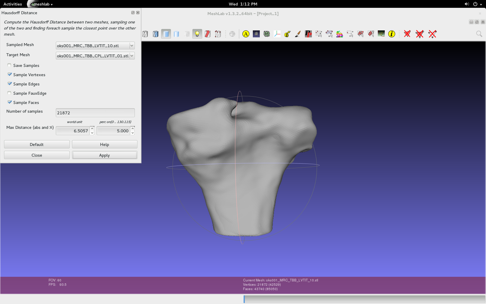
Filters > Sampling > Hausdorff Distance.
- Use the default values specific to the imported geometries, as seen in the image below.
- Either can be the target or sampled mesh, but make sure to repeat and switch.
Filters > Color Creation and Processing > Colorize by Vertex Quality.
- Use the default values specific to the imported geometries, as shown in below image.
- In addition, choose the appropriate percentile crop value. If not zero this value will be used for a percentile cropping of the quality values. If this parameter is set to P the value V for which P% of the vertices have a quality lower (greater) than V is used as min (max) value. The automated percentile cropping is very useful for automatically discarding outliers.
- Min: The value that will be mapped with the lower end of the scale (blue).
- Max: The value that will be mapped with the upper end of the scale (red).
- Note that they're relative. Using two different master volumes for segmentation (cartilage versus general purpose) can skew data because general purpose has a larger image and would have error in the regions not contained in the cartilage image.

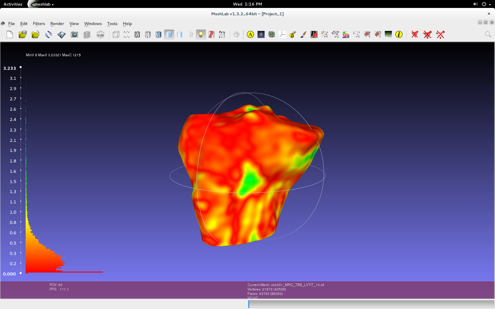
- Play with show layer dialogue in order to see just the layer (geometry/mesh) that was colorized.
- The geometry that was selected as the sampled mesh will be colored.
Render > Show Vert Quality Histogram
- For later reference, take a screenshot of the colored geometry, without a transparent background. Also, the geometry can be exported as a .ply file, retaining the vertex quality and color. Further, the log can be saved by copying the text into a .txt file. The naming convention is as followed:
For log, GeometryObject_SampledAuthorInitials_TargetAuthorInitials.txt
- Ex., FMB_CPL_CB.txt
For .ply, GeometryObject_SampledAuthorInitials_TargetAuthorInitials_PercentCrop.ply
- Ex., FMB_CPL_CB_05.ply
For snapshot, GeometryObject_SampledAuthorInitials_TargetAuthorInitials_PercentCrop.png
- Ex., FMB_CPL_CB_05.png
- Note that this naming convention is temporary and could be subject to change. Currently, the specimen number (oks00#) is not included because all results will already be under that folder.
Results
The results from the comparisons can be found within the repository at oks/oks001/dat/Geometry/Comparison Results, or by clicking on this link.
There are three folders and a readme file. The logs folder contains the logs as .txt files for each comparison. These log files were created by copy and pasting the information in the meshlab log into a .txt file. The rms values can be found here. Furthermore, the meshes folder contains the .ply files for each comparison. The snapshots folder contains screenshots for each comparison.
Examples
Comparing Identical Geometries
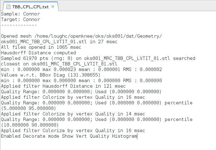
Below is an example of the same geometry compared with itself. Notice that there is very little, if no error present. However, when the percentile crop is changed from 0 to 5, the color scheme quickly changes. Regardless, the lack of error shows the Hausdorf Distance method is an accurate technique when measuring how identical two geometries are.
Example of Log file from Comparison:
Comparison with Percentile Crop of 0:
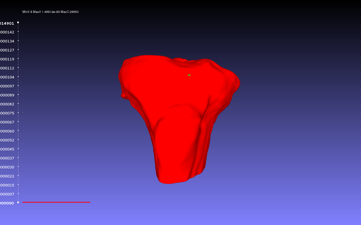
Comparison with Percentile Crop of 5:

Comparison with Percentile Crop of 10:
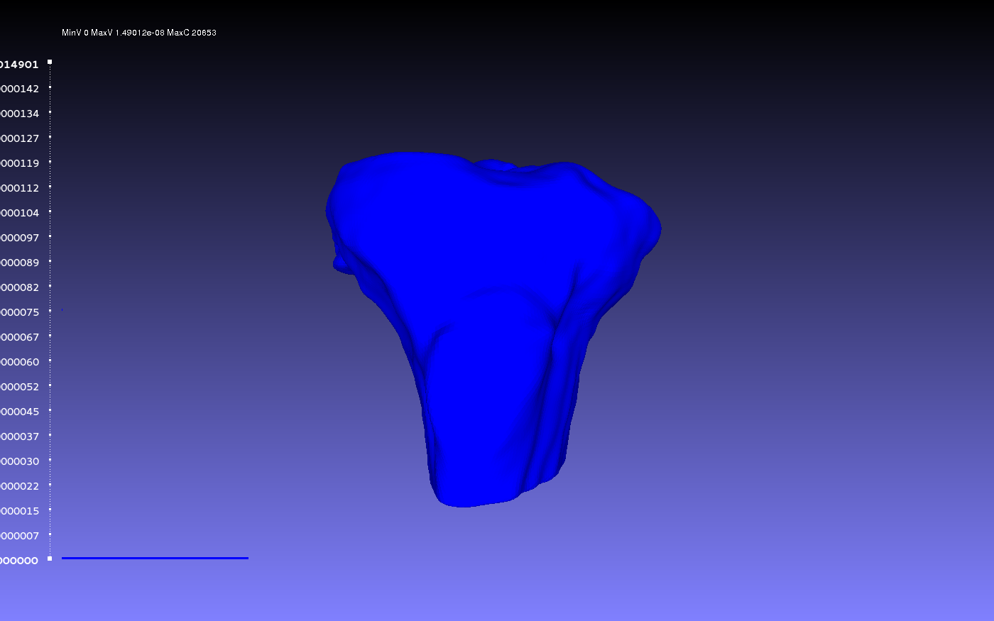
Comparing Raw versus Smooth
Below is an example of a raw tibia bone compared to the resulting smoothed version. The smoothing was done according to the guidelines outlines on the GeometryGeneration page. The example shows when smoothed bone was the sampled geometry (left) and when it was the target geometry (right).
Percentile Crop of 0:
 vs.
vs. 
Percentile Crop of 5:
 vs.
vs. 
Percentile Crop of 10:
 vs.
vs. 
Percentile Crop of 15:
 vs.
vs. 
Percentile Crop of 20:
 vs.
vs. 
Comparing Two Smoothed Geometries
Below is an example of a two smoothed tibia bones compared, one by the author CPL and one by the author CB. Such a comparison can show how similarly the two authors segmented the tibia. For both authors, the smoothing was done according to the guidelines outlines on the GeometryGeneration page. The example shows when CPL's smoothed tibia bone was the sampled geometry (left) and when it was the target geometry (right).
Percentile Crop of 0:
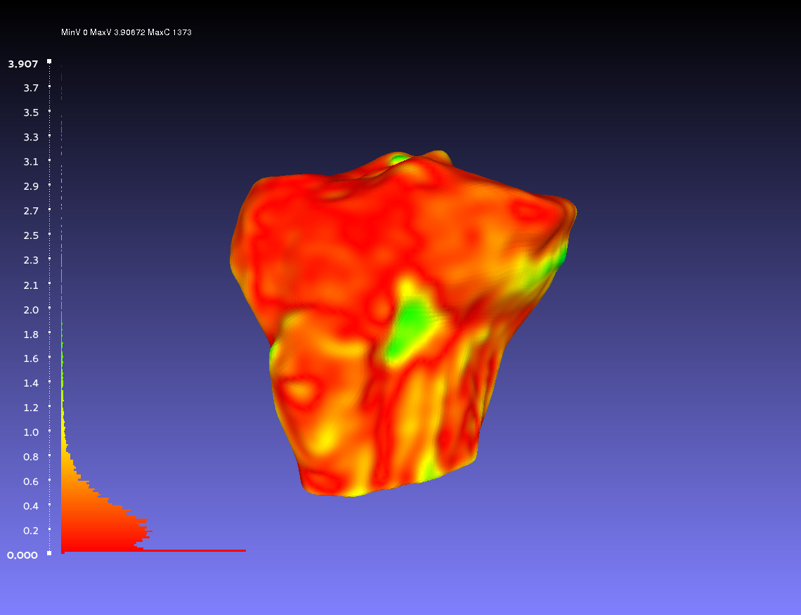 vs.
vs. 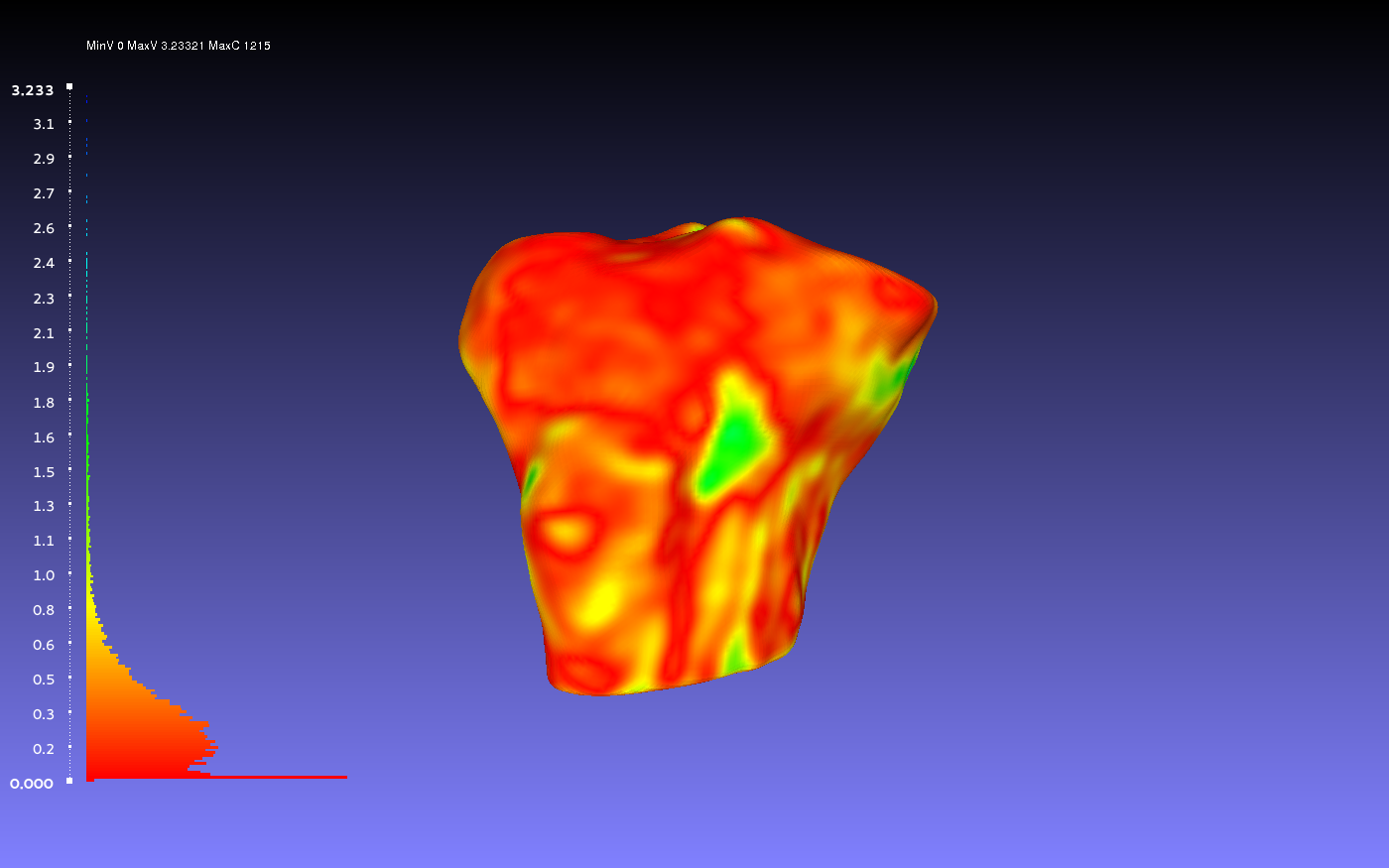
Percentile Crop of 5:
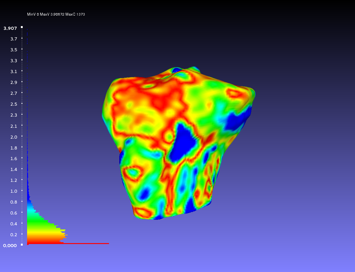 vs.
vs. 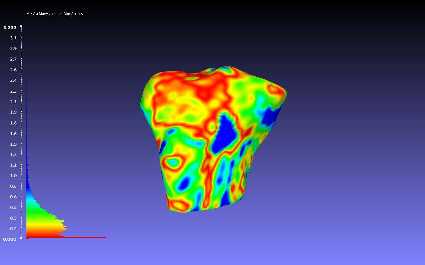
Percentile Crop of 10:
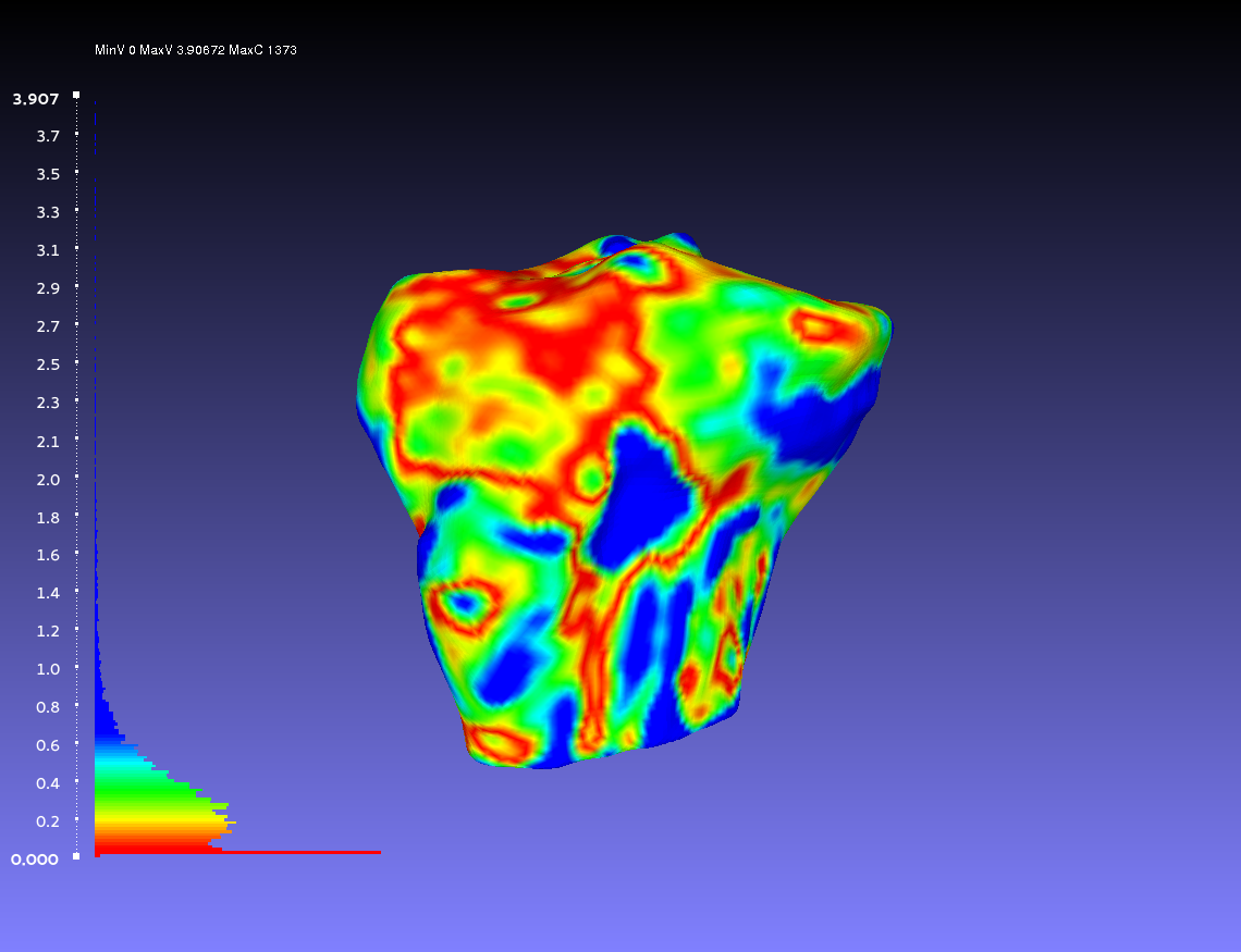 vs.
vs. 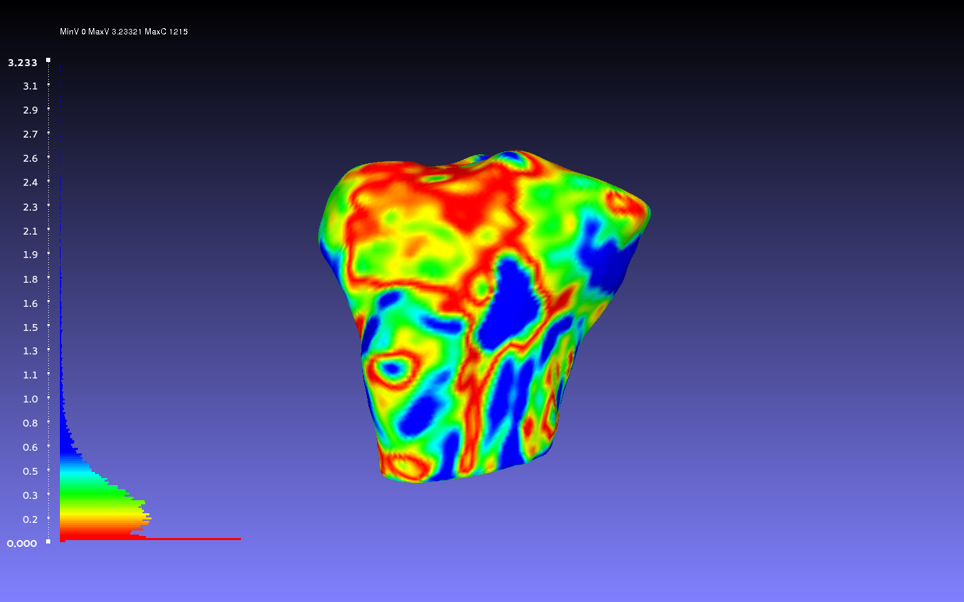
Percentile Crop of 15:
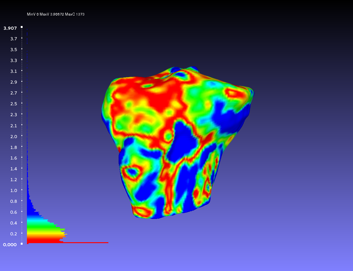 vs.
vs. 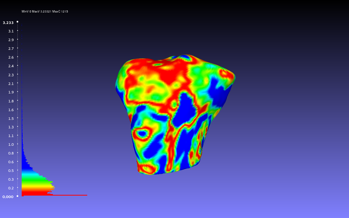
Percentile Crop of 20:
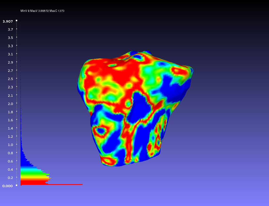 vs.
vs. 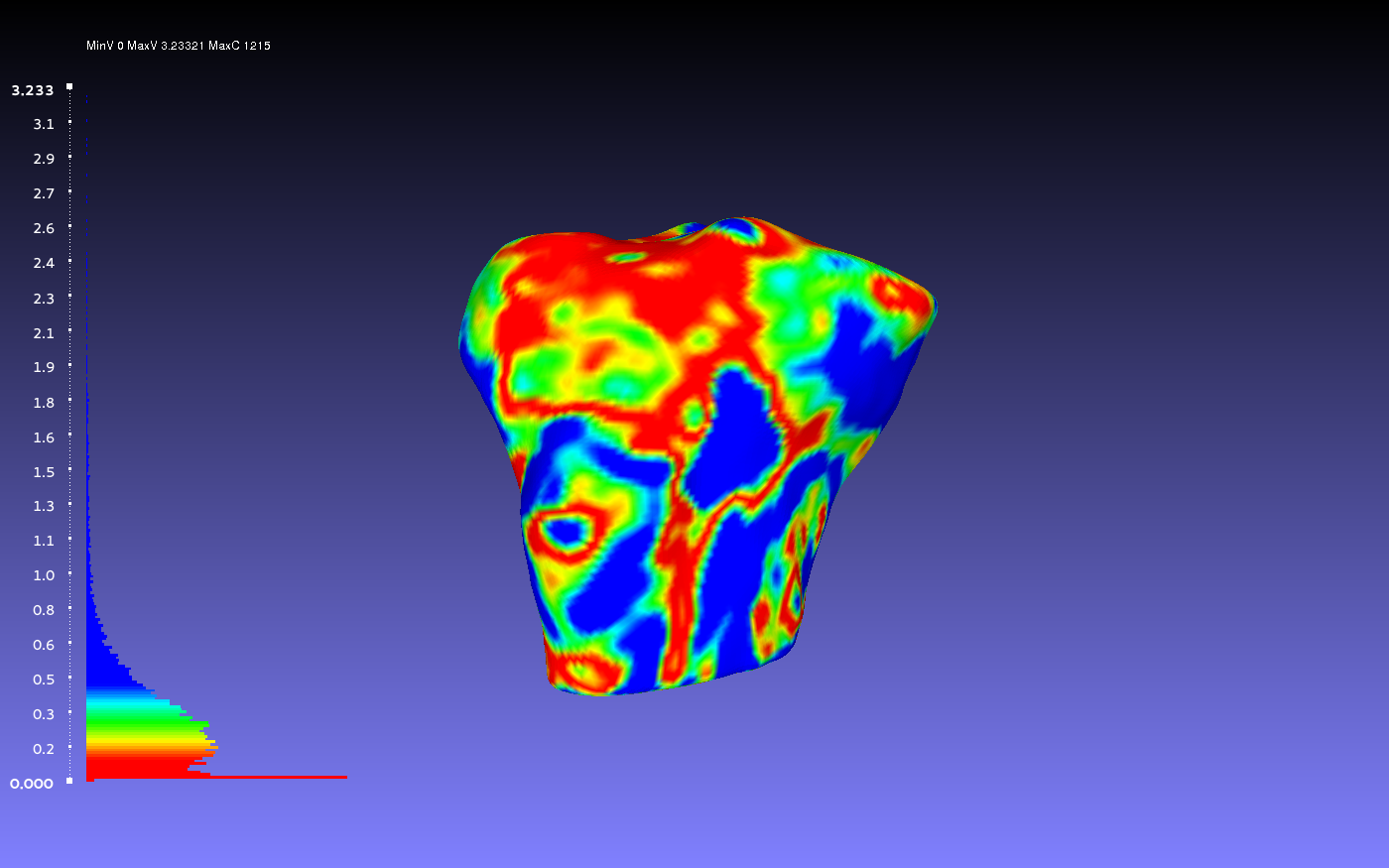
Automating Meshlab
MeshLabServer
Meshlabserver is MeshLab’s automated component. Unfortunately, there documentation on meshlabserver is limited. Meshlabserver has been incorporated into the automated smoothing and geometry comparison scripts, with the goal of minimizing time spent on repetitive processes.
Below is a screenshot image of the information provided when accessing meshlab server through the terminal.
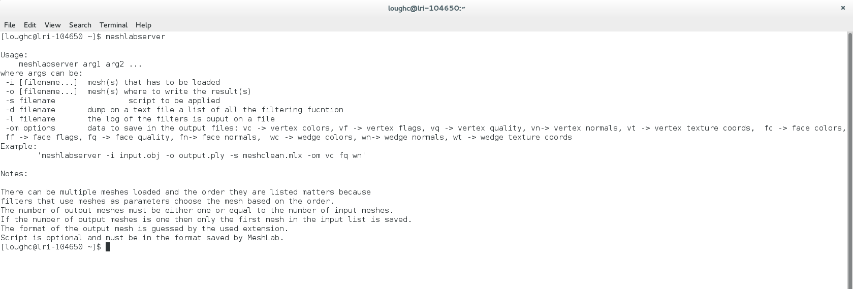
An example using meshlabserver for geometry smoothing:
meshlabserver -i oks001_MRG_FBB_CPL_RAW_01.stl -o result2.stl -s MeshLab_FBB_Smooth_1.mlx -l log2.txt
Above, the input file is oks001_MRG_FBB_CPL_RAW_01.stl, the output file is result2.stl, the script used is MeshLab_FBB_Smooth_1.mlx, and the log is log2.txt.
Additionally, an example of using meshlabserver for geometry comparison:
meshlabserver -i oks001_MRC_TBB_LVTIT_10.stl oks001_MRC_TBB_CPL_LVTIT_01.stl -o Comparison Results/Meshes/results.ply -s MeshLab_Comparison.mlx -l log1.txt
Where oks001_MRC_TBB_LVTIT_10.stl and oks001_MRC_TBB_CPL_LVTIT_01.stl are the input files, Comparison Results/Meshes/results.ply is the output file, and the script for the process is MeshLab_Comparison.mlx. Additionally, a log of the process will be stored in log1.txt.
Creating Filter Scripts
More information to come...
oks/oks001/dat/Geometry/Scripts.pdf
For Smoothing
More information to come...
oks/oks001/dat/Geometry/Geo_Smooth.py
oks/oks001/dat/Geometry/DetermineValues.py
oks/oks001/dat/Geometry/MlxWriter.py
oks/oks001/dat/Geometry/MeshlabServerCaller.py
oks/oks001/dat/Geometry/MeshLab_FBB_Smooth_1.mlx
oks/oks001/dat/Geometry/MeshLab_FBB_Smooth_2.mlx
oks/oks001/dat/Geometry/MeshLab_PTB_Smooth.mlx
oks/oks001/dat/Geometry/MeshLab_TBB_FMB_Smooth.mlx
For Comparison
More information to come...
oks/oks001/dat/Geometry/Geo_Compare.py
oks/oks001/dat/Geometry/MeshLab_Comparison.mlx
oks/oks001/dat/Geometry/DetermineValues.py
oks/oks001/dat/Geometry/MlxWriter.py
oks/oks001/dat/Geometry/MeshlabServerCaller.py
References
Rote, G. (1991). Computing the minimum Hausdorff distance between two point sets on a line under translation. Information Processing Letters, 38(3), 123-127. doi:10.1016/0020-0190(91)90233-8
Huttenlocher, D., Klanderman, G., & Rucklidge, W. (1993, September). Comparing images using the Hausdorff distance. IEEE Transactions on Pattern Analysis and Machine Intelligence IEEE Trans. Pattern Anal. Machine Intell., 15(9), 850-863. PDF Link
