Differences between revisions 53 and 54

Contents

Target Outcome
Prerequisites
1. Infrastructure
2. Previous Protocols
Comparing Two Geometries
Automating Meshlab
References

Target Outcome

To compare two geometries and determine how consistent they are with one another. Ultimately, the end goal is to generate a colorized geometry that, based on its color, indicates to what degree the particular geometry resembles another.

Prerequisites

Infrastructure

MeshLab. MeshLab is an open source, portable, and extensible system for the processing and editing of unstructured 3D triangular meshes (GPL license, see http://meshlab.sourceforge.net/).

Previous Protocols

For more information, see:

Comparing Two Geometries

Background: Hausdorff Distance

Hausdorff distance is defined as the "maximum distance of a set to the nearest point in another set." [Rote] This distance essentially "measures the extent to which each point of a 'model' set lies near some point of an 'image' set, and vice versa." [Huttenlocher] With that being said, the Hausdorff distance can be used to "determine the degree of resemblance when two objects are superimposed on one another." [Huttenlocher] With two geometries, the Hausdorff distance is dependent upon which geometries is selected as the target geometry and which is selected as the sampled geometry. For analysis, the following process should be done with the two geometries as both the target and sampled geometries (mesh) to ensure an accurate comparison. In other words, the process should be repeated and the geometries (meshes) should be switched.

Process

Load both .stl geometry files into Meshlab.
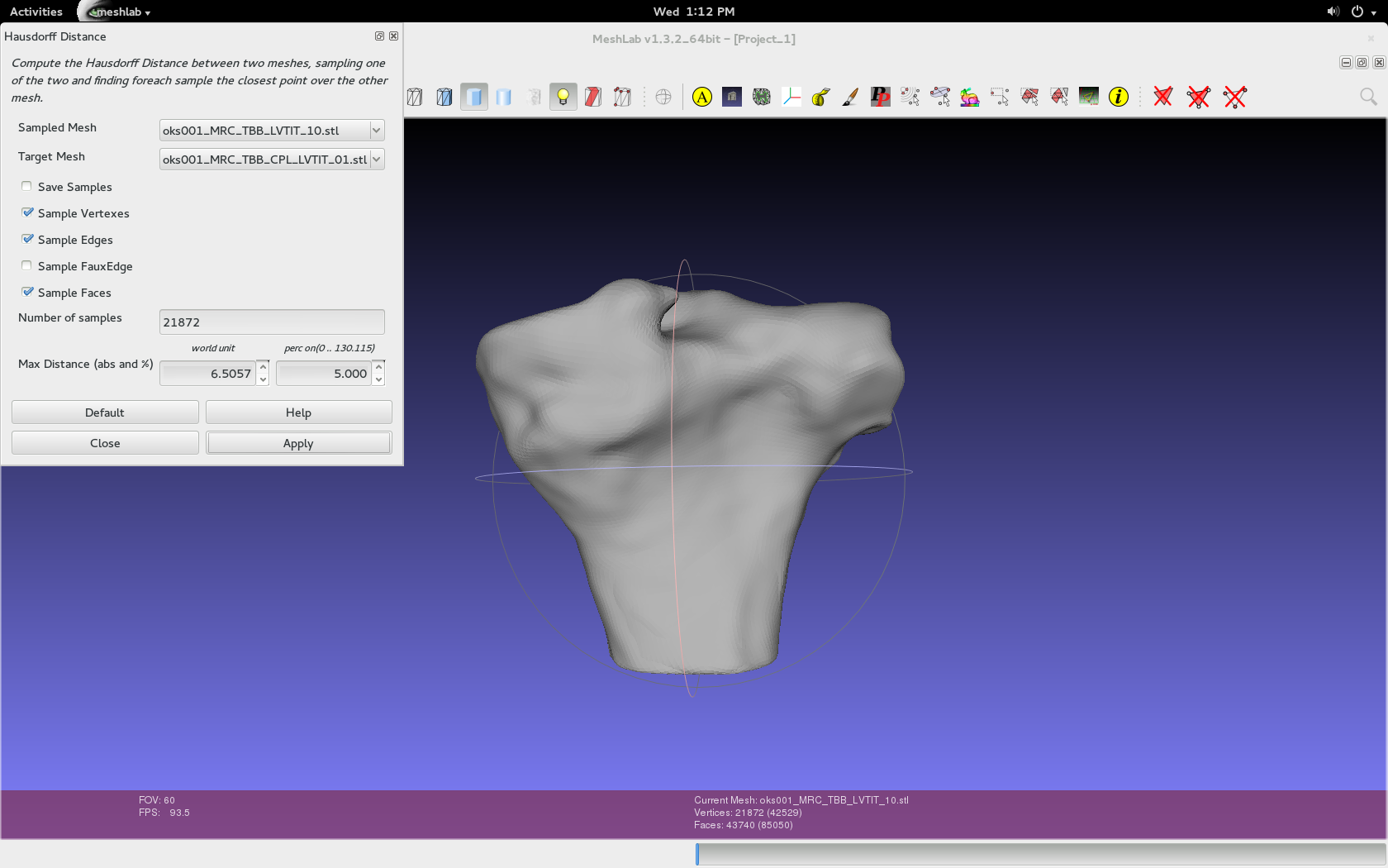
Filters > Sampling > Hausdorff Distance.
- Use the default values specific to the imported geometries, as seen in the image below.
- Either can be the target or sampled mesh, but make sure to repeat and switch.
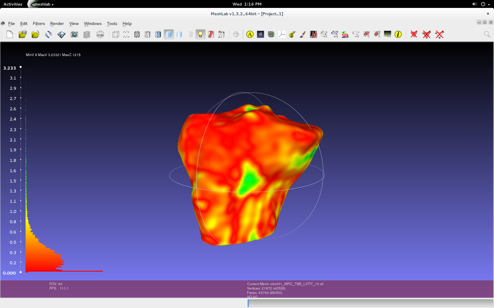
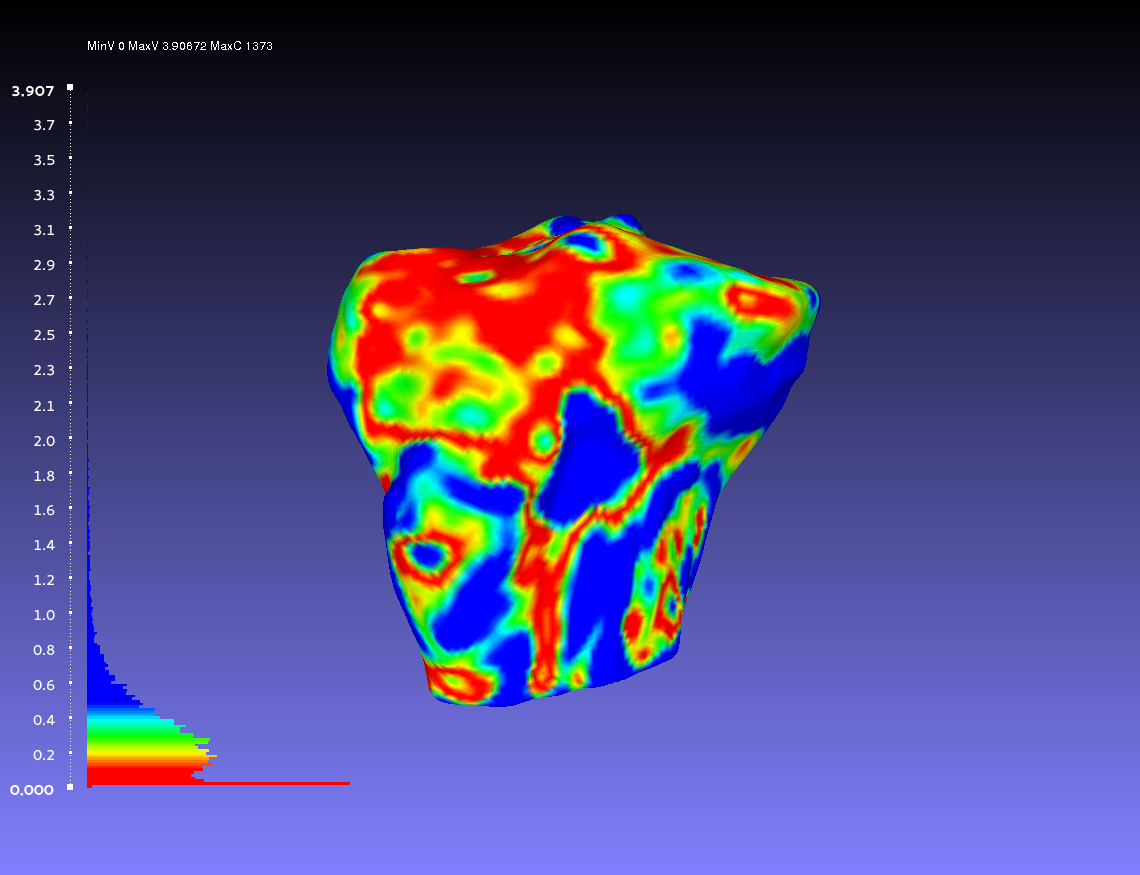
Filters > Color Creation and Processing > Colorize by Vertex Quality.
- Use the default values specific to the imported geometries, as shown in below image.
- In addition, choose the appropriate percentile crop value. If not zero this value will be used for a percentile cropping of the quality values. If this parameter is set to P the value V for which P% of the vertices have a quality lower (greater) than V is used as min (max) value. The automated percentile cropping is very useful for automatically discarding outliers.
- Min: The value that will be mapped with the lower end of the scale (blue).
- Max: The value that will be mapped with the upper end of the scale (red).
- Note that they're relative. Using two different master volumes for segmentation (cartilage versus general purpose) can skew data because general purpose has a larger image and would have error in the regions not contained in the cartilage image.
Play with show layer dialogue in order to see just the layer (geometry/mesh) that was colorized.
- The geometry that was selected as the sampled mesh will be colored.
Render > Show Vert Quality Histogram
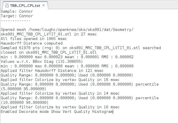
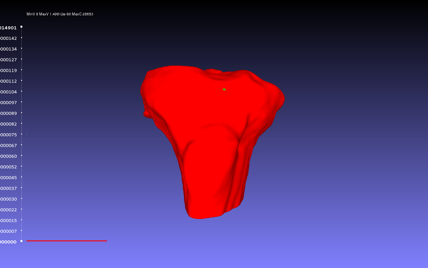
For later reference, take a screenshot of the colored geometry, without a transparent background. Also, the geometry can be exported as a .ply file, retaining the vertex quality and color. Further, the log can be saved by copying the text into a .txt file. The naming convention is as followed:
- For log, (Geometry Object)_(Sampled Author Initials)_(Target Author Initials).txt
  - Ex., FMB_CPL_CB.txt
- For .ply, (Geometry Object)_(Sampled Author Initials)_(Target Author Initials)_(Percent Crop).ply
  - Ex., FMB_CPL_CB_05.ply
- For snapshot, (Geometry Object)_(Sampled Author Initials)_(Target Author Initials)_(Percent Crop).png
  - Ex., FMB_CPL_CB_05.png

Examples

Comparing Identical Geometries

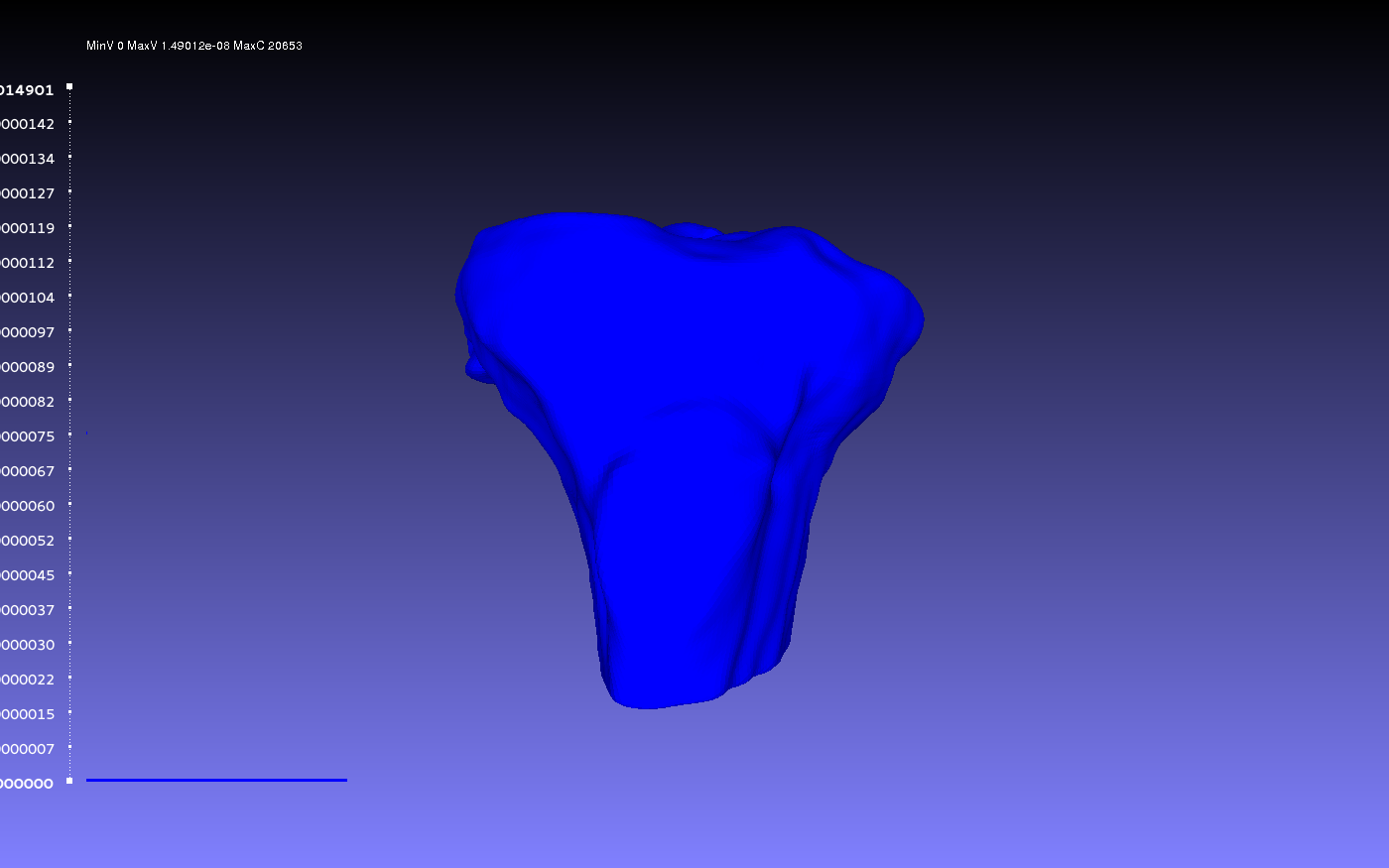
Comparing Raw versus Smooth

vs.

Comparing Two Smoothed Geometries

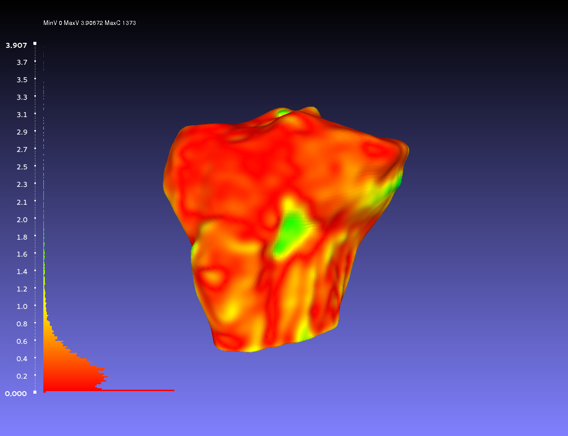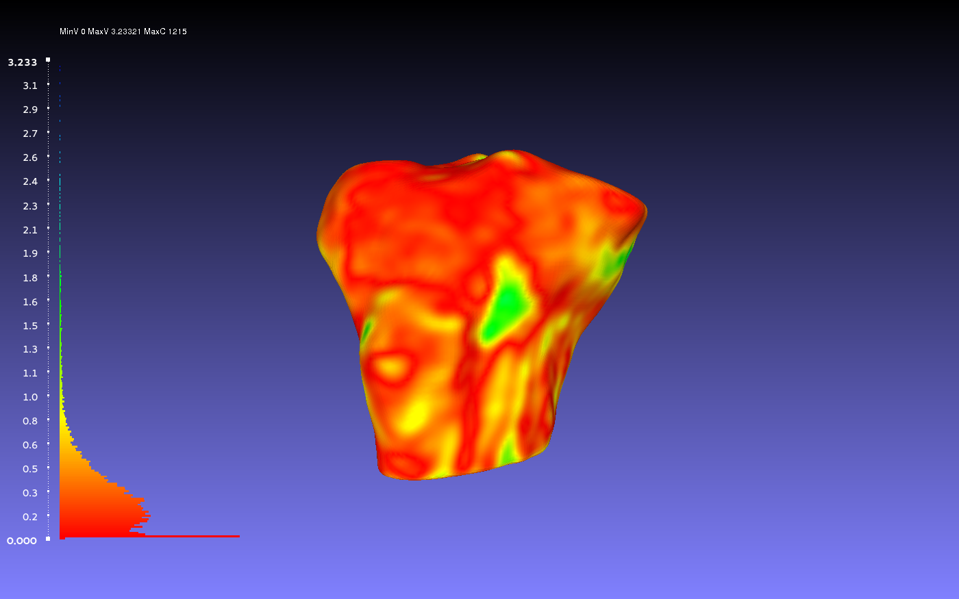
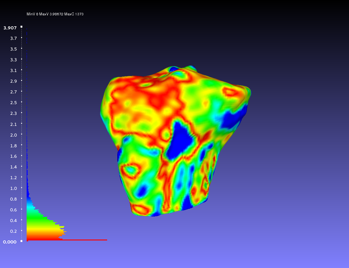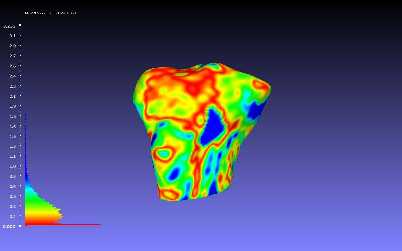
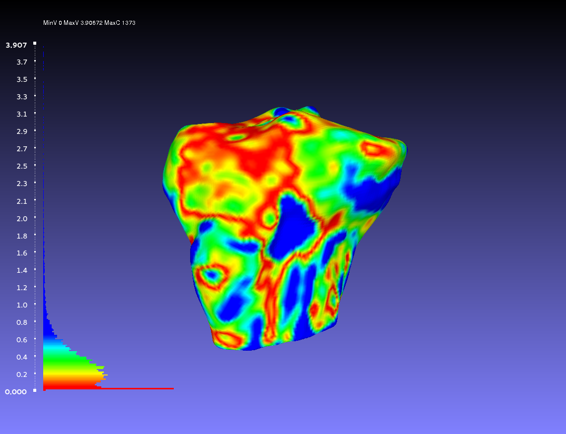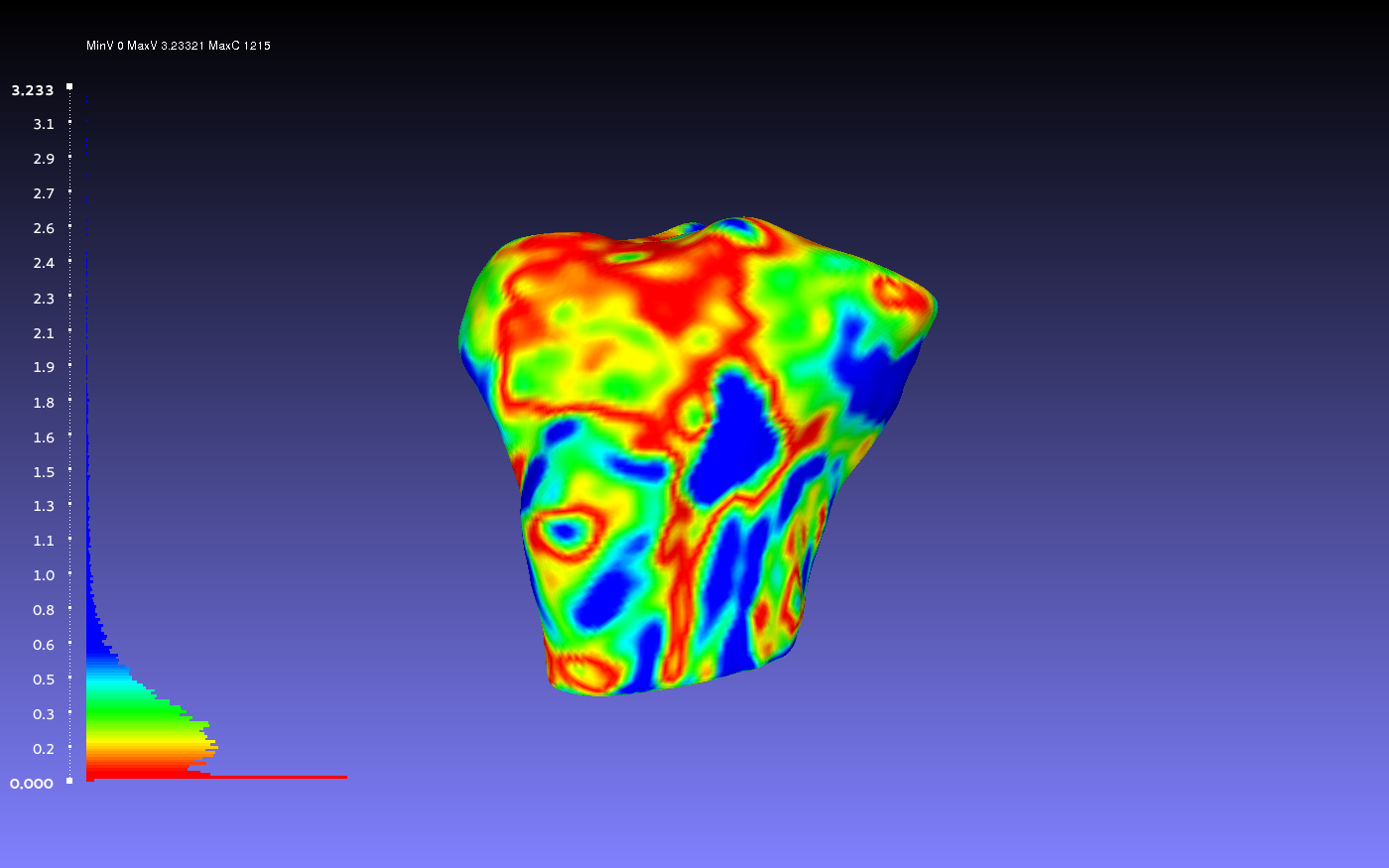
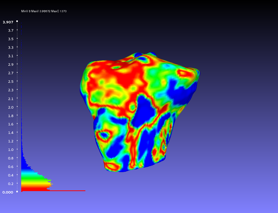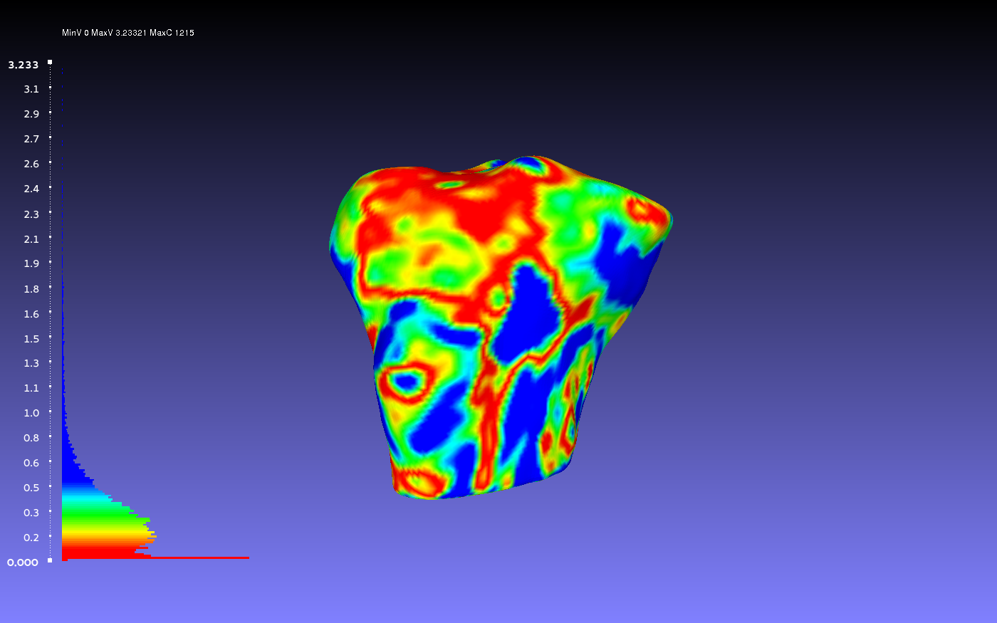
vs.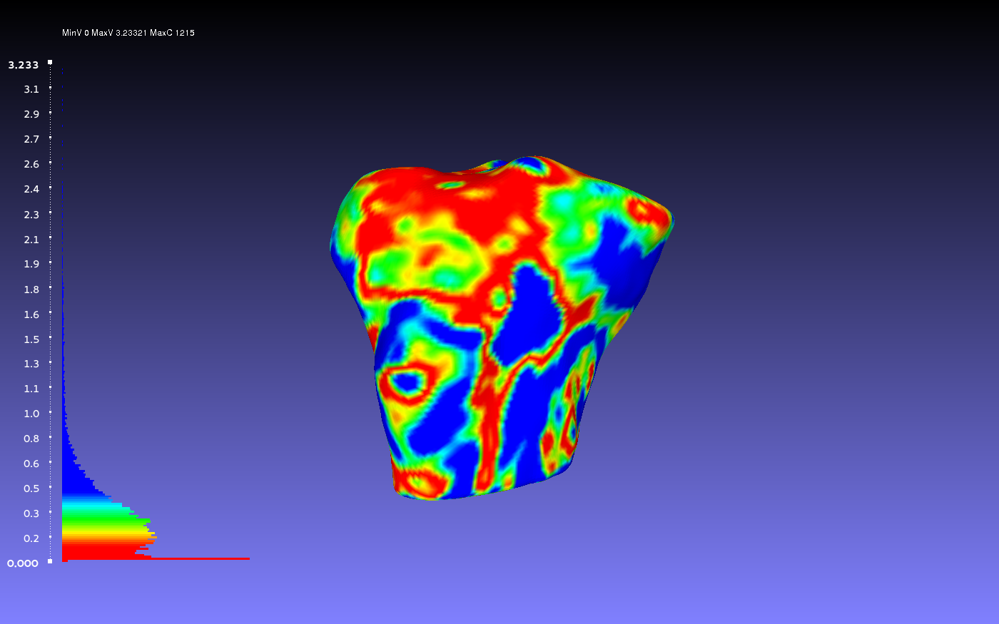

Automating Meshlab

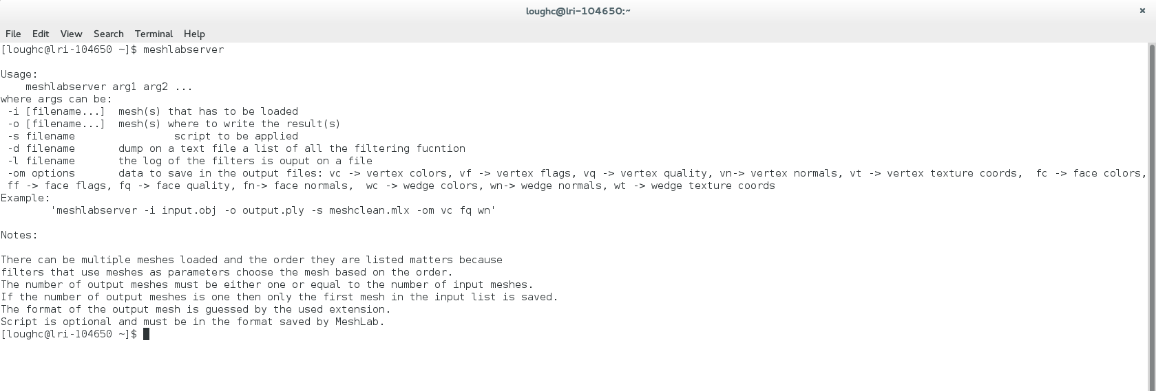
MeshLabServer

More information to come...

Creating Filter Scripts

More information to come...

For Smoothing

More information to come...

oks/oks001/dat/Geometry/MeshLab_Commands.txt

oks/oks001/dat/Geometry/MeshLab_FBB_Smooth.mlx

oks/oks001/dat/Geometry/MeshLab_PTB_Smooth.mlx

oks/oks001/dat/Geometry/MeshLab_TBB_FMB_Smooth.mlx

For Comparison

More information to come...

oks/oks001/dat/Geometry/MeshLab_Comparison.mlx

examples ... oks/oks001/dat/Geometry/MeshLab_Commands.txt

results ... oks/oks001/dat/Geometry/Comparison Results

References

G. Rote (1991). Computing the minimum Hausdorff distance between two point sets on a line under translation. Information Processing Letters, v. 38, pp. 123-127.

Huttenlocher DP, Klanderman GA, Rucklidge WJ. Comparing Images Using the Hausdorff Distance. IEEE Transactions on Pattern Analysis and Machine Intelligence. 1993 September; Vol. 15, No. 9, pg 850. PDF Link

-  ⇤ ← Revision 53 as of 2016-07-25 19:21:50 → 
  Size: 6819
  Editor: mentalwealth
  Comment:
+   ← Revision 54 as of 2016-07-25 19:37:59 → ⇥
  Size: 6427
  Editor: mentalwealth
  Comment:
-Deletions are marked like this.
+Additions are marked like this.
 Line 7:
-Line 13:
+Line 12:
 Line 18:
-Line 20:
+Line 19:
-Line 24:
+Line 22:
-Line 27:
+Line 24:
-    * Use the default values specific to the imported geometries, as seen in the image below.
    * Either can be the target or sampled mesh, but make sure to repeat and switch.

    {{attachment:hausdorff.png|hausdorff.png|width=500}}
+  * Use the default values specific to the imported geometries, as seen in the image below.
  * Either can be the target or sampled mesh, but make sure to repeat and switch.
  {{attachment:hausdorff.png||width="500"}}
-Line 33:
+Line 29:
-    * Use the default values specific to the imported geometries, as shown in below image.
    * In addition, choose the appropriate percentile crop value. If not zero this value will be used for a percentile cropping of the quality values. If this parameter is set to P the value V for which P% of the vertices have a quality lower (greater) than V is used as min (max) value. The automated percentile cropping is very useful for automatically discarding outliers.
    * Min: The value that will be mapped with the lower end of the scale (blue).
    * Max: The value that will be mapped with the upper end of the scale (red).
    * Note that they're relative. Using two different master volumes for segmentation (cartilage versus general purpose) can skew data because general purpose has a larger image and would have error in the regions not contained in the cartilage image.

    {{attachment:colorize.png|colorize.png|width=500}}
+  * Use the default values specific to the imported geometries, as shown in below image.
  * In addition, choose the appropriate percentile crop value. If not zero this value will be used for a percentile cropping of the quality values. If this parameter is set to P the value V for which P% of the vertices have a quality lower (greater) than V is used as min (max) value. The automated percentile cropping is very useful for automatically discarding outliers.
  * Min: The value that will be mapped with the lower end of the scale (blue).
  * Max: The value that will be mapped with the upper end of the scale (red).
  * Note that they're relative. Using two different master volumes for segmentation (cartilage versus general purpose) can skew data because general purpose has a larger image and would have error in the regions not contained in the cartilage image.
  {{attachment:colorize.png||width="500"}}
-Line 42:
+Line 37:
-    * The geometry that was selected as the sampled mesh will be colored.
+  * The geometry that was selected as the sampled mesh will be colored.
-Line 44:
+Line 39:
-    {{attachment:final.png|final.png|width=500}}
+  . {{attachment:final.png||width="500"}}
-Line 48:
+Line 42:
-    * For log, (Geometry Object)_(Sampled Author Initials)_(Target Author Initials).txt
      * Ex., FMB_CPL_CB.txt
    * For .ply, (Geometry Object)_(Sampled Author Initials)_(Target Author Initials)_(Percent Crop).ply
      * Ex., FMB_CPL_CB_05.ply
    * For snapshot, (Geometry Object)_(Sampled Author Initials)_(Target Author Initials)_(Percent Crop).png
      * Ex., FMB_CPL_CB_05.png
+  * For log, (Geometry Object)_(Sampled Author Initials)_(Target Author Initials).txt
   * Ex., FMB_CPL_CB.txt
  * For .ply, (Geometry Object)_(Sampled Author Initials)_(Target Author Initials)_(Percent Crop).ply
   * Ex., FMB_CPL_CB_05.ply
  * For snapshot, (Geometry Object)_(Sampled Author Initials)_(Target Author Initials)_(Percent Crop).png
   * Ex., FMB_CPL_CB_05.png
-Line 57:
+Line 50:
-Line 59:
+Line 51:
-{{attachment:log.png|log.png|width=800}}
{{attachment:TBB_CPL_CPL_00.png|TBB_CPL_CPL_00.png|width=500}}
{{attachment:TBB_CPL_CPL_05.png|TBB_CPL_CPL_05.png|width=500}}
{{attachment:TBB_CPL_CPL_10.png|TBB_CPL_CPL_10.png|width=500}}
+{{attachment:log.png||width="800"}} {{attachment:TBB_CPL_CPL_00.png||width="500"}} {{attachment:TBB_CPL_CPL_05.png||width="500"}} {{attachment:TBB_CPL_CPL_10.png||width="500"}}
-Line 66:
+Line 54:
+{{attachment:TBB_CPL_LVTIT_CPL_RAW_00.png||width="300"}} vs. {{attachment:TBB_CPL_RAW_CPL_LVTIT_00.png||width="300"}}
-Line 67:
+Line 56:
-{{attachment:TBB_CPL_LVTIT_CPL_RAW_00.png|TBB_CPL_LVTIT_CPL_RAW_00.png|width=300}} vs. {{attachment:TBB_CPL_RAW_CPL_LVTIT_00.png|TBB_CPL_RAW_CPL_LVTIT_00.png|width=300}}
+{{attachment:TBB_CPL_LVTIT_CPL_RAW_05.png||width="300"}} vs. {{attachment:TBB_CPL_RAW_CPL_LVTIT_05.png||width="300"}}
-Line 69:
+Line 58:
-{{attachment:TBB_CPL_LVTIT_CPL_RAW_05.png|TBB_CPL_LVTIT_CPL_RAW_05.png|width=300}} vs. {{attachment:TBB_CPL_RAW_CPL_LVTIT_05.png|TBB_CPL_RAW_CPL_LVTIT_05.png|width=300}}
+{{attachment:TBB_CPL_LVTIT_CPL_RAW_10.png||width="300"}} vs. {{attachment:TBB_CPL_RAW_CPL_LVTIT_10.png||width="300"}}
-Line 71:
+Line 60:
-{{attachment:TBB_CPL_LVTIT_CPL_RAW_10.png|TBB_CPL_LVTIT_CPL_RAW_10.png|width=300}} vs. {{attachment:TBB_CPL_RAW_CPL_LVTIT_10.png|TBB_CPL_RAW_CPL_LVTIT_10.png|width=300}}
+{{attachment:TBB_CPL_LVTIT_CPL_RAW_15.png||width="300"}} vs. {{attachment:TBB_CPL_RAW_CPL_LVTIT_15.png||width="300"}}
-Line 73:
+Line 62:
-{{attachment:TBB_CPL_LVTIT_CPL_RAW_15.png|TBB_CPL_LVTIT_CPL_RAW_15.png|width=300}} vs. {{attachment:TBB_CPL_RAW_CPL_LVTIT_15.png|TBB_CPL_RAW_CPL_LVTIT_15.png|width=300}}

{{attachment:TBB_CPL_LVTIT_CPL_RAW_20.png|TBB_CPL_LVTIT_CPL_RAW_20.png|width=300}} vs. {{attachment:TBB_CPL_RAW_CPL_LVTIT_20.png|TBB_CPL_RAW_CPL_LVTIT_20.png|width=300}}
+{{attachment:TBB_CPL_LVTIT_CPL_RAW_20.png||width="300"}} vs. {{attachment:TBB_CPL_RAW_CPL_LVTIT_20.png||width="300"}}
-Line 78:
+Line 65:
+{{attachment:TBB_CPL_CB_00.png||width="300"}} vs. {{attachment:TBB_CB_CPL_00.png||width="300"}}
-Line 79:
+Line 67:
-{{attachment:TBB_CPL_CB_00.png|TBB_CPL_CB_00.png|width=300}} vs. {{attachment:TBB_CB_CPL_00.png|TBB_CB_CPL_00.png|width=300}}
+{{attachment:TBB_CPL_CB_05.png||width="300"}} vs. {{attachment:TBB_CB_CPL_05.png||width="300"}}
-Line 81:
+Line 69:
-{{attachment:TBB_CPL_CB_05.png|TBB_CPL_CB_05.png|width=300}} vs. {{attachment:TBB_CB_CPL_05.png|TBB_CB_CPL_05.png|width=300}}
+{{attachment:TBB_CPL_CB_10.png||width="300"}} vs. {{attachment:TBB_CB_CPL_10.png||width="300"}}
-Line 83:
+Line 71:
-{{attachment:TBB_CPL_CB_10.png|TBB_CPL_CB_10.png|width=300}} vs. {{attachment:TBB_CB_CPL_10.png|TBB_CB_CPL_10.png|width=300}}
+{{attachment:TBB_CPL_CB_15.png||width="300"}} vs. {{attachment:TBB_CB_CPL_15.png||width="300"}}
-Line 85:
+Line 73:
-{{attachment:TBB_CPL_CB_15.png|TBB_CPL_CB_15.png|width=300}} vs. {{attachment:TBB_CB_CPL_15.png|TBB_CB_CPL_15.png|width=300}}

{{attachment:TBB_CPL_CB_20.png|TBB_CPL_CB_20.png|width=300}} vs. {{attachment:TBB_CB_CPL_20.png|TBB_CB_CPL_20.png|width=300}}
+{{attachment:TBB_CPL_CB_20.png||width="300"}} vs. {{attachment:TBB_CB_CPL_20.png||width="300"}}
-Line 90:
+Line 76:
+== MeshLabServer ==
More information to come...
-Line 91:
+Line 79:
-== MeshLabServer ==
+{{attachment:terminal.png||width="500"}}
-Line 93:
+Line 81:
-{{attachment:terminal.png|terminal.png|width=500}}
+== Creating Filter Scripts ==
More information to come...
-Line 96:
+Line 85:
+More information to come...
-Line 106:
+Line 96:
-oks/oks001/dat/Geometry/MeshLab_Commands.txt

oks/oks001/dat/Geometry/Comparison Results
+More information to come...
-Line 113:
+Line 100:
+examples ... oks/oks001/dat/Geometry/MeshLab_Commands.txt

results ... oks/oks001/dat/Geometry/Comparison Results
-Line 114:
+Line 105:
-Line 117:
+Line 107:
-Huttenlocher DP, Klanderman GA, Rucklidge WJ. Comparing Images Using the Hausdorff Distance. IEEE Transactions on Pattern Analysis and Machine Intelligence. 1993 September; Vol. 15, No. 9, pg 850. [[https://www.cs.cornell.edu/~dph/papers/HKR-TPAMI-93.pdf| PDF Link]]
+Huttenlocher DP, Klanderman GA, Rucklidge WJ. Comparing Images Using the Hausdorff Distance. IEEE Transactions on Pattern Analysis and Machine Intelligence. 1993 September; Vol. 15, No. 9, pg 850. [[https://www.cs.cornell.edu/~dph/papers/HKR-TPAMI-93.pdf|PDF Link]]