|
Size: 14584
Comment:
|
Size: 14584
Comment:
|
| Deletions are marked like this. | Additions are marked like this. |
| Line 206: | Line 206: |
| * [[attachment:ThicknessComparison_MRI_US.odp|Initial comparison of US and MRI]] | * [[attachment:ThicknessComparison_MRI_US.pdf|Initial comparison of US and MRI]] |
Target Outcome
Prerequisites
Protocols
File Association
- Setting up the Directory
- Download and unpack the subject folder and place in MULTIS_trials folder
- The folder/file configuration should be the following
MULTIS_trials
MULTIS###-# (Subject folder containing all data)
Configuration - Configuration files and subject XML
Data - All "tdms" files
Ultrasound - All "dicom" files
PulseWidths300.csv - contains key to decode file association pulse
manualMatcherFA.py
plotterFA.py
XMLparser.py
dataAnalysis.py
tdsmParserMultis.py
- Running the File Association script
- Install libraries as needed
- Change Directory to match desired Subject ID
- Ensure Plot is True to save all verification plots
- Run script.
- Check directory in file browser under the subject folder for the following additions
- FileAssociationPNG - folder
TimeSynchronization.txt - file containing trial numbers and delta T's of accepted trials only
- MULTIS###-#readme.txt - human readable file which summarizes the file matching
- Manually Matching
- Open the 'MULTIS###-#readme.txt' file
- Note the Unmatched and Accepted Trials, specifically the binary column
- Examine any files beginning with 'NMa', meaning no match found
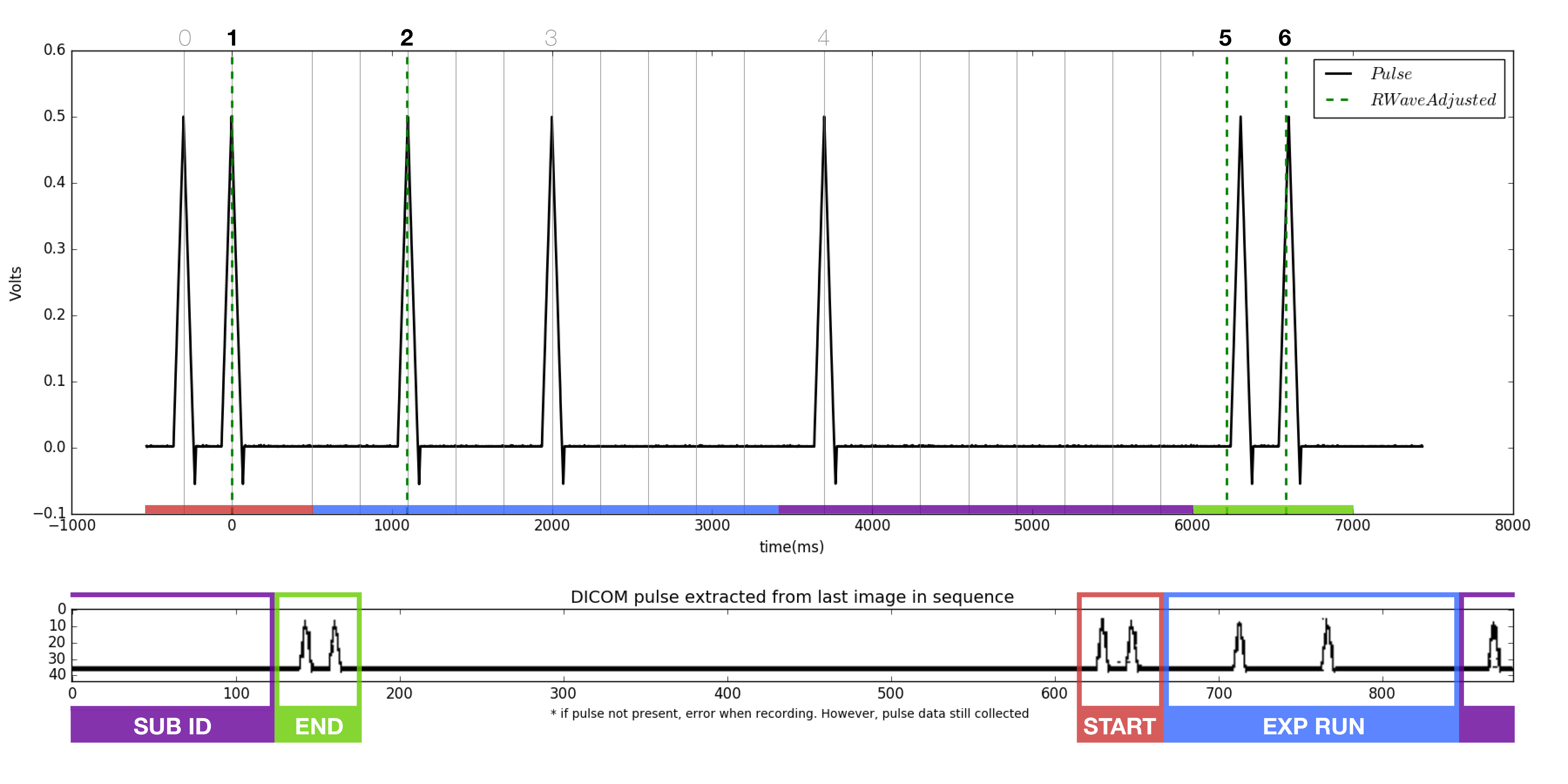
- Locate the start and end pluses, each a burst of two peaks.
- Compare the binary of the trial run number to each of the pulse sequences found in the 'NMa' png's. Note the file names of each. At this point, it is known which file each of the missing accepted trial numbers belong to.
Open the manualMatcherFA.py and plotterFA.py python scripts.
Change the directory file names in the manualMatcherFA script to a pair of matching files found in step 2. Only one pair of files will be compared at a time. The files will be imported to the plotterFA script automatically.
- Run the plotterFA.py script, ensuring iteration is set to zero.
- Examine the figure generated.
- The pulse extracted from the dicom (bottom of figure) should match the pulse from the tdms file (top of figure). Note the dicom pulse will not always begin at the left most portion of the window as it is a continuous loop in the ultrasound machine.
- As before, locate the beginning and ending double pulses.
- Count the number of peaks present in the dicom pulse.
- Count the number of RWaves in the generated figure.
- It is likely that one or more of the RWaves are missing, as that is why the files did not match.
- Change the iteration from 0, to 1, to 2, and so on and re-plot each time until the RWaves appear to line up with the pulse peaks in the top figure.
- Identify which peaks have RWaves, and which do not.
- Each of the peaks in the upper figure has a number associated with it in the script. Starting from 0, instead of 1, the peaks are named accordingly.
- Record which peaks have RWaves. For example. (1,2,5,6) may have RWaves.
- Open the 'MULTIS###-#readme.txt' file

9 . Return to manualMatcherFA.py
- Ensure iteration is set to 2.
- Change the chosenRwaves variable to reflect the the recorded RWaves i.e. (1,2,5,6)
- Run the script
- Check the following items
- The filename of the dicom and tdms changed appropriately
- The trial number and time synch were added to
MULTIS###-#readme.txt
The updated PNG was added to the FileAssociationPNG folder
Quality Assurance
- Setting up the Directory
- same as file association with the addition of folders created by file association
- Running the dataAnalysis.py script
- Change Directory to reflect subject ID
- Run script
- Check the following
A folder named AnalysisPNG should appear under MULTIS###-#
- 56 png files should be found within this folder
- Analysis
- There are two types of figures
- Anatomical
- 3 dicom images (at 1st pulse, minimum force, last pulse) over load cell data
- Indentation
- 4 dicom images (at pre, start, middle, max indentation) over load cell data
- Anatomical
- There are two types of figures


Thickness Measurements
Version 1.0 places red circles at the coordinates of the previous frame that was analyzed, starting with the second frame. Version 1.1 moves red circles to the location with the closest matched distribution to the coordinates in the previous frame, starting with the second frame. Version 2.0 does not require the user to hit 'enter' to save the thicknesses and allows the user to cycle through all of the locations for one subject instead of restarting the program after each location.
- Setting up the Directory
- Download and unpack the desired Subject ID folder, make sure you use the 'associated' data if you do not want to associate the files yourself.
Note: If you have just completed the file association, confirm that the dicom and tdms files within the Ultrasound and Data folders have been matched (should begin with a three digit number) and that the corresponding deltaT values (as xml files) are located in the TimeSynchronization folder.
- Download and unpack the desired Subject ID folder, make sure you use the 'associated' data if you do not want to associate the files yourself.
- The folder/file configuration should be the following
MULTIS###-# (Subject folder containing all data - the required data for the thickness measurements is shown below)
Configuration - Contains subject xml file for accepted trials
Data - Contains tdms files
Ultrasound - Contains dicom files
TimeSynchronization - Contains xml files with deltaT values for matched trials
- Required Python scripts
TA_sfm_v#.#.py
tdsmParserMultis.py
XMLparser.py
Plot_thicknessForce.py
- Running the manual thickness measurement script
- Install libraries as needed
- Change the directory to match where the Python scripts are located
- Run script
- The first dialog window will allow you to select the Subject folder (you may also choose to hard code the path to the Subject folder, found within the getFiles() function)
- Browse through to find the location of this folder and click 'ok'
- A list will appear in another window which will show all the trials for that subject (you may have to scroll down to see the entire list)
- Double-click on the location you would like to analyze
- After a couple of seconds, the first image will appear
- The program behaves differently depending on if the trial is anatomical or indentation
- Anatomical - The program begins with the frame corresponding to the lowest resultant force
- Indentation - The program begins with the frame that corresponds to the beginning of indentation
- The program behaves differently depending on if the trial is anatomical or indentation
- Drag the red dots so that the center of the dot is over each boundary (use the built in matplotlib toolbar to zoom in if needed)
- Transducer/Skin boundary
- Skin/Fat boundary
- Fat/Muscle boundary
- Muscle/Bone boundary
- When you are happy with your selection, press 'next image' and the results will be calculated and saved to an xml file.
- The next frame for analysis will automatically appear
- Anatomical trials will give you the image corresponding to the next lowest force, until all frames within the first pulse and last pulse range have been analyzed
- Indentation trials will give you the next image in the sequence until reaching the maximum force
- After analyzing the frames for that location, hit the 'Done' button and the list of images for that subject will re-appear and you can analyze a new location.
- The xml file that was saved will be re-formatted using pretty print (only if you hit the 'Done' button)
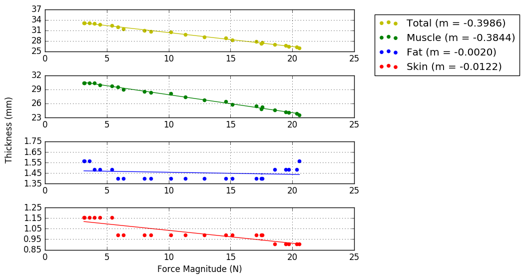
A PNG folder within the Analysis folder will be created that has saved images of the first frame that was analyzed as well as a graph showing the force/thickness relationships
- You may end the program at any time by clicking the 'X' button in the upper right hand corner.
- All windows will be closed and the script will stop running

- All windows will be closed and the script will stop running
- The first dialog window will allow you to select the Subject folder (you may also choose to hard code the path to the Subject folder, found within the getFiles() function)
- Data storage
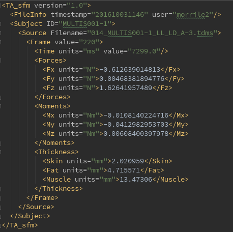
- The xml file will be named using the tdms filename with '_manThick'+ time stamp appended
- Version of software used for analysis (TA_sfm.py)
- File Info includes the time stamp at the beginning of analysis as well as the user name at the time of program execution
- Subject shows the MULTIS ID name
- Source shows the Filename of the data (tdms) file
- A new 'Frame' child is appended for each frame that is analyzed
- The Frame child includes the following information:
- Value - Frame number
- Time - Reference time from the ultrasound time vector data (in ms)
- Forces - Forces in the x, y, and z directions (in N)
- Moments - Moments in the x, y, and z directions (in Nm)
- Thicknesses - Skin, Fat, and Muscle layers (in mm)
- The Frame child includes the following information:
- The xml file will be named using the tdms filename with '_manThick'+ time stamp appended
Multiple Subject Summary
- Demographics summary
- What you will need
- subject_demographics_summary.py
- Subject xml files to include in the summary
- Running the summary script
- Program will search for 'MULTIS_test' directory, if it cannot find that directory you will be asked to browse for the directory.
- A list of available subjects will appear, check the boxes of the subjects that you would like to include in the summary (use the 'Select All' button to automatically select all boxes)
- Click 'Okay' and the script will run
A figure with all of the data will appear, refer to the attached example figure and key with the description of variables. Demographics Summary Examplekey.png
- What you will need
- Thickness summary (anatomical trials only)
- What you will need
- subject_thickness_summary.py
- Thickness xml files to include in the summary in appropriate analysis folder
- Running the summary script
- Program will search for 'MULTIS_test' directory, if it cannot find that directory you will be asked to browse for the directory.
- A list of available subjects will appear, check the boxes of the subjects that you would like to include in the summary (use the 'Select All' button to automatically select all boxes)
- Click 'Okay' and the script will run
A figure for each location (16 total) will be saved in a folder called ThickSumFigs. Thickness Summary Example
- What you will need
Repeatability & Reproducibility
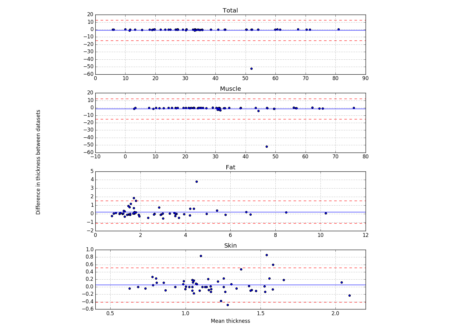
Bland & Altman plots (example below) showing the thicknesses of the first frame of each location that was analyzed (Plot_thicknessForce_reliability_ALL.py)
- Blue line shows the mean difference
- Red lines show 2 standard deviations above and below the mean difference
- Script outputs the trial number of the differences that are further than 2 standard deviations from the mean difference.
Results for reproducibility of MULTIS004 (Rici and Ahmet both analyzed all anatomical trials). Bland Altman Plot

Automated Thickness Measurement Development
- Note: The automated development has been suspended until data is collected on additional subjects.
- Texture analysis of boundaries (transducer/skin, skin/fat, fat/muscle, and muscle/bone)
- Extract rectangles (3mm x 6mm) with boundary located in center
- Analyze by regions
- Fit to a Gaussian curve (average horizontally and then normalize by peak intensity)
- Examine moments of the image using skimage.measure module (Hu's moments, first invariant is analogous to moment of inertia)
Initial results report (using 12 locations from MULTIS-001-1): report1.pdf
Preliminary Results/Questions
In Vivo Thickness Analysis
Report for radiologist examination. Thickness Analysis Questions for Radiologist
- Meeting notes with Dr. Delzell (2016-11-21)
- Images with unsure bone boundaries were difficult to determine if it was bone or fascia, Dr. Delzell suggests using the transverse imaging mode to find the bone first and then switching to the longitudinal mode to capture our images.
- When looking for the boundary of fat to muscle, the fascia of the muscle should be clearly defined by a bright signal (if in the correct plane)
- Many of the distal locations have little to no fat
See Thickness Analysis Comments from Dr. Delzell for more comments relating to specific images.
- Meeting notes with Dr. Delzell (2016-11-21)
In Vitro Ultrasound/MRI Thickness Comparison
Trial 1
- MRI: Trial 4, Ultrasound: MULTIS_C_008-1
- Used ITK snap to estimate MRI thicknesses
- There are quite a few discrepancies between the two imaging modalities
- Initial thoughts:
- Consistency in position of leg between Ultrasound and MRI - Potentially a stand for the head of the femur
- Positions (proximal, central, distal, medial, lateral, anterior, posterior) from the MRI may not match the positions of the Ultrasound - this will be improve once Optotrak is implemented
- Concern with consistency between in vivo and in vitro experimentation - Tyler will work with Tammy to learn the in vivo protocol and apply it to in vitro
- Improvements needed:
- Consistency between ultrasound of in vivo and in vitro
- Consistency between ultrasound and MRI of the in vivo extremities


