 |
API
4.0
For C++ developers
|
 |
API
4.0
For C++ developers
|
This is a class that acts as a user friendly wrapper to QuinticBezerCurveSet to build specific kinds of physiologically plausible muscle curves using C2 continuous sets of quintic Bezier curves.
More...
Static Public Member Functions | |
| static SmoothSegmentedFunction * | createFiberActiveForceLengthCurve (double lce0, double lce1, double lce2, double lce3, double minActiveForceLengthValue, double plateauSlope, double curviness, bool computeIntegral, const std::string &curveName) |
This is a function that will produce a C2 (continuous to the second derivative) active force length curve. More... | |
| static SmoothSegmentedFunction * | createFiberForceVelocityCurve (double fmaxE, double dydxC, double dydxNearC, double dydxIso, double dydxE, double dydxNearE, double concCurviness, double eccCurviness, bool computeIntegral, const std::string &curveName) |
This function will generate a C2-continuous (continuous to the second derivative) force velocity curve of a single muscle fiber. More... | |
| static SmoothSegmentedFunction * | createFiberForceVelocityInverseCurve (double fmaxE, double dydxC, double dydxNearC, double dydxIso, double dydxE, double dydxNearE, double concCurviness, double eccCurviness, bool computeIntegral, const std::string &muscleName) |
This function will generate a C2-continuous (continuous to the 2nd derivative) inverse curve that the function createFiberForceVelocityCurve generates. More... | |
| static SmoothSegmentedFunction * | createFiberCompressiveForcePennationCurve (double phi0, double kiso, double curviness, bool computeIntegral, const std::string &curveName) |
This element will generate a C2-continuous (continuous to the 2nd derivative) compressive force profile curve as a function of pennation. More... | |
| static SmoothSegmentedFunction * | createFiberCompressiveForceCosPennationCurve (double cosPhi0, double kiso, double curviness, bool computeIntegral, const std::string &curveName) |
This element will generate a C2-continuous (continuous to the 2nd derivative) compressive force profile curve as a function of cos(pennation). More... | |
| static SmoothSegmentedFunction * | createFiberCompressiveForceLengthCurve (double l0, double kiso, double curviness, bool computeIntegral, const std::string &curveName) |
This element will generate a C2-continuous (continuous to the second derivative) curve that models a compressive force profile that is a function of fiber length. More... | |
| static SmoothSegmentedFunction * | createFiberForceLengthCurve (double eZero, double eIso, double kLow, double kIso, double curviness, bool computeIntegral, const std::string &curveName) |
This function will generate a C2-continuous curve that fits a fiber's tensile force length curve. More... | |
| static SmoothSegmentedFunction * | createTendonForceLengthCurve (double eIso, double kIso, double fToe, double curviness, bool computeIntegral, const std::string &curveName) |
Will generate a C2-continuous (continuous to the second derivative) curve in a MuscleFunctionObject object that fits a tendon's tensile force length curve. More... | |
This is a class that acts as a user friendly wrapper to QuinticBezerCurveSet to build specific kinds of physiologically plausible muscle curves using C2 continuous sets of quintic Bezier curves.
This class has been written there did not exist a set of curves describing muscle characteristics that was:
1. Physiologically Accurate
2. Continuous to the second derivative
3. Parameterized in a physically meaningful manner
For example, the curves employed by Thelen (Thelen DG(2003). Adjustment of Muscle Mechanics Model Parameters to Simulate Dynamic Contractions in Older Adults. ASME Journal of Biomechanical Engineering (125).) are parameterized in a physically meaningful manner, making them easy to use. However there are many shortcomings of these curves:
a. The tendon and parallel element are not C2-continuous, making them slow to simulate and likely not physiologically accurate. b. The active force length curve approaches does not achieve its minimum value at a normalized fiber length of 0.5, and 1.5. c. The force velocity curve is not C2-continuous at the origin. As it is written in the paper the curve is impossible to use with an equilibrium model because it is not invertible. In addition the force-velocity curve actually increases in stiffness as activation drops - a very undesirable property given that many muscles are inactive at any one time.
The muscle curves used in the literature until 2012 have been hugely influenced by Thelen's work, and thus similar comments can easily be applied to just about every other musculoskeletal simulation.
Another example is from Miller (Miller,RH(2011).Optimal Control of Human Running. PhD Thesis). On pg 149 a physiologically plausible force velocity curve is specified that gives the user the ability to change the concentric curvature to be consistent with a slow- or a fast-twitch muscle. This curve is not C2-continuous at the origin, but even worse, it contains singularities in its parameter space. Since these parameters do not have a physical interpretation this model is difficult to use without accidentally creating a curve with a singularity.
With this motivation I set out to develop a class that could generate muscle characteristic curves with the following properties:
1. Physiologically Accurate
2. Continuous to the second derivative
3. Parameterized in a physically meaningful manner
4. Monotonicity for monotonic curves
5. Computationally efficient
These goals were surprisingly difficult to achieve, but these goals have been achieved using sets of C2-continuous quintic Bezier curves. The resulting muscle curve functions in this class take parameters that would be intuitive to biomechanists who simulate human musculoskeletal systems, and returns a SmoothSegmentedFunction which is capable of evaluating the value, derivatives and optionally the integral of the desired function (or actually relation as the case may be).
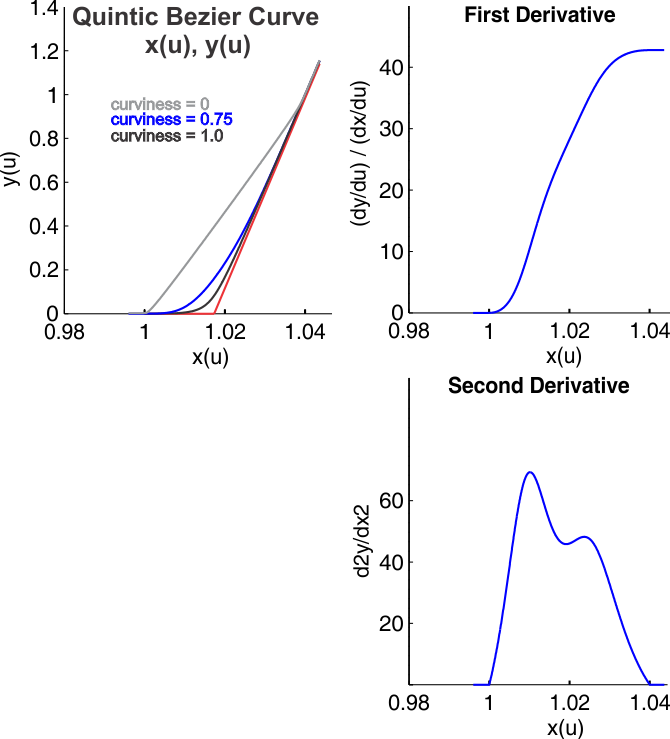
Each curve is made up of one or more C2 quintic Bezier curves x(u), and y(u), with linearly extrapolated ends as shown in the figure below. These quintic curves span 2 points, and achieve the desired derivative at its end points. The degree of curviness can be varied from 0 to 1 (0, 0.75 and 1.0 are shown in the figure in gray, blue and black respectively), and will make the curve approximate a line when set to 0 (gray), and approximate a curve that hugs the intersection of the lines that are defined by the end points locations and the slopes at the end of each curve segment (red lines). Although you do not need to set all of this information directly, for some of the curves it is useful to know that both the slope and the curviness parameter may need to be altered to achieve the desired shape.
Computational Cost Details All computational costs assume the following operation costs:
Operation Type     : #flops
*,+,-,=,Boolean Op : 1
                 / : 10
               sqrt: 20
               trig: 40
These relative weightings will vary processor to processor, and so any of the quoted computational costs are approximate.
|
static |
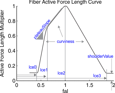
This is a function that will produce a C2 (continuous to the second derivative) active force length curve.
| lce0 | Normalized fiber length at the left-most shoulder of the active force-length curve. The value of the active force length curve for lce < lce0 will be equal to the value set in shoulderVal. Normally lce0 is approximately 0.5 |
| lce1 | Normalized fiber length at the transition point between the ascending limb and the plateau region of the active force length curve. |
| lce2 | Normalized fiber length at the maximum active force length curve value of 1. Normally lce2 is by definition 1. |
| lce3 | Normalized fiber length of the at the right most shoulder of the active-force length curve. The value of the active force length curve for lce > lce2 will be equal to the value of shoulderVal. Normally lce3 is approximately 1.5 |
| minActiveForceLengthValue | The minimum value of the active force length curve. A physiological non-equilibrium muscle model would have this value set to 0. An equilibrium muscle model would have a non-zero lower bound on this value of 0.1 typically. shoulderVal must be greater than, or equal to 0. |
| plateauSlope | The slope of the plateau of the active force length curve between lce1 and lce2. This parameter can vary depending on the muscle model, but a value of 0.8616 is a good place to start. |
| curviness | The dimensionless 'curviness' parameter that can vary between 0 (a line) to 1 (a smooth, but sharply bent elbow). A value of 0 will yield an active force length curve that is composed of slightly curved line segments. A value of 1 will yield an active force length curve that is smoothly rounded. |
| computeIntegral | If this is true, the integral for this curve is numerically calculated and splined. If false, this integral is not computed, and a call to .calcIntegral will throw an exception |
| curveName | The name of the muscle this curve applies to. This curve name should have the name of the muscle and the curve in it (e.g. "bicep_fiberActiveForceLengthCurve") so that, if this curve ever causes an exception, a user-friendly error message can be displayed to the end user to help them debug their model. |
| SimTK::Exception | if these conditions aren't met -0 < lce0 < lce1 < lce2 < lce3 -shoulderVal >= 0 -0 <= plateauSlope < (1/(lce3-lce2)) -0 <= curviness <= 1 |
Conditions:
Computational Costs
    Without Integral :   ~20,500 flops
    With Integral    :  ~870,500 flops
Example:
|
static |
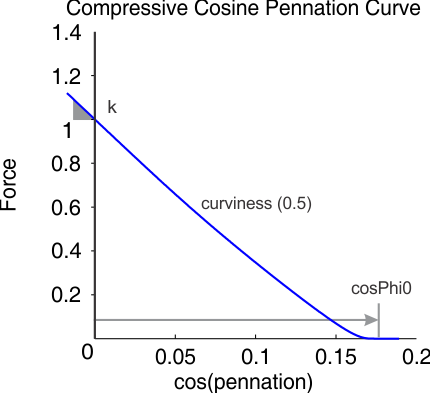
This element will generate a C2-continuous (continuous to the 2nd derivative) compressive force profile curve as a function of cos(pennation).
A muscle model with this element usually places this element in line with the tendon. The main function of this element is to prevent the fiber from achieving a pennation angle of pi/2 radians. This type of element is necessary for a parallelogram pennated muscle models because without it, the muscle model can deform to the point where a pennation angle of pi/2 radians is reached, which causes a singularity in the model.
| cosPhi0 | The cosine of the pennation angle at which the compressive force element starts to engage. When the cos of the pennation angle is greater than cosPhi0, the compressive element generates no force. When cos of the pennation angle is less than cosPhi0, the compressive element generates a compressive force. |
| kiso | This is the maximum stiffness of the compressive element, which occurs when cosPhi is zero. This parameter must be negative cos |
| curviness | The dimensionless 'curviness' parameter that can vary between 0 (a line) to 1 (a smooth, but sharply bent elbow) |
| computeIntegral | If this is true, the integral for this curve is numerically calculated and splined. If false, this integral is not computed, and a call to .calcIntegral will throw an exception |
| curveName | The name of the muscle this curve applies to. This curve name should have the name of the muscle and the curve in it (e.g. "bicep_fiberCompressiveForceCosPennationCurve") so that, if this curve ever causes an exception, a user-friendly error message can be displayed to the end user to help them debug their model. |
| SimTK::Exception | unless the following conditions are met: -0 < cosPhi0 -kiso > 1/(cosPhi0) -0 <= curviness <= 1 |
Computational Costs
    Without Integral :   ~4,100 flops
    With Integral    : ~174,100 flops
Example:
|
static |
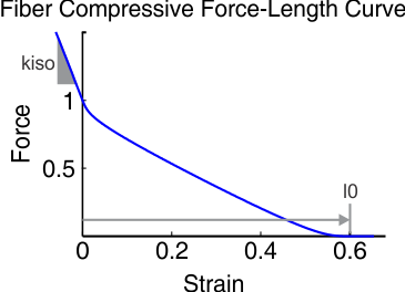
This element will generate a C2-continuous (continuous to the second derivative) curve that models a compressive force profile that is a function of fiber length.
The main function of this element is to prevent the fiber from achieving an unrealistically short length. This type of element is necessary for equilibrium-type muscle models because of the editing that is done to the active force length curve that endows an equilibrium model fiber with the ability to to generate force when a physiological fiber cannot.
| l0 | The normalized fiber length at which the compressive element starts to engage. When the fiber is shorter than l0, the compressive element is generating a force. When the fiber length is longer than l0, the compressive element generates no force. |
| kiso | This is the maximum stiffness of the compressive element, which occurs when the fiber has a length of 0, under a load of 1 maximum isometric unit of force. |
| curviness | The dimensionless 'curviness' parameter that can vary between 0 (a line) to 1 (a smooth, but sharply bent elbow) |
| computeIntegral | If this is true, the integral for this curve is numerically calculated and splined. If false, this integral is not computed, and a call to .calcIntegral will throw an exception |
| curveName | The name of the muscle this curve applies to. This curve name should have the name of the muscle and the curve in it (e.g. "bicep_fiberCompressiveForceLengthCurve") so that, if this curve ever causes an exception, a user-friendly error message can be displayed to the end user to help them debug their model. |
| SimTK::Exception | unless the following conditions are met -e0 > 0 -kiso > 1/(e0) -0 <= curviness <= 1 |
Computational Costs
    Without Integral :   ~4,100 flops
    With Integral    : ~174,100 flops
Example:
|
static |
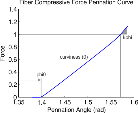
This element will generate a C2-continuous (continuous to the 2nd derivative) compressive force profile curve as a function of pennation.
A muscle model with this element usually places this element parallel to the fiber.The main function of this element is to prevent the fiber from achieving a pennation angle of pi/2 radians. This type of element is necessary for a parallelogram pennated equilibrium muscle models because without it, the muscle model can deform to the point where a pennation angle of pi/2 radians is reached, which causes a singularity in the model.
| phi0 | The pennation angle at which the compressive force element starts to engage . When the pennation angle is greater than phi0, the compressive element is generating a force. When the pennation angle is less than phi0, the compressive element generates no force. |
| kiso | This is the maximum stiffness of the compressive element, which occurs when the fiber is pennated by 90 degrees |
| curviness | The dimensionless 'curviness' parameter that can vary between 0 (a line) to 1 (a smooth, but sharply bent elbow) |
| computeIntegral | If this is true, the integral for this curve is numerically calculated and splined. If false, this integral is not computed, and a call to .calcIntegral will throw an exception |
| curveName | The name of the muscle this curve applies to. This curve name should have the name of the muscle and the curve in it (e.g. "bicep_fiberCompressiveForcePennationCurve") so that, if this curve ever causes an exception, a user-friendly error message can be displayed to the end user to help them debug their model. |
| SimTK::Exception | unless the following conditions are met -0 < phi0 < SimTK::Pi/2 -kiso > 1/(SimTK::Pi/2-phi0) -0 <= curviness <= 1 |
Computational Costs
    Without Integral :   ~4,100 flops
    With Integral    : ~174,100 flops
Example:
|
static |
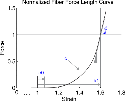
This function will generate a C2-continuous curve that fits a fiber's tensile force length curve.
| eZero | The fiber strain at which the fiber begins to develop force. Thus an e0 of 0.0 means that the fiber will start to develop passive force when it has a normalized length of 1.0. Note that e0 can be positive or negative. |
| eIso | The fiber strain at which the fiber develops 1 unit of normalized force (1 maximum isometric force). Note that the '1' is left off. Thus an e0 of 0.6 means that the fiber will develop an 1 normalized force unit when it is strained by 60% of its resting length, or to a normalized length of 1.6 |
| kLow | The normalized stiffness (or slope) of the fiber curve close to the location where the force-length curve approaches a normalized force of 0. This is usually chosen to be a small, but non-zero fraction of kIso (kLow = 0.025 kIso is typical). |
| kIso | The normalized stiffness (or slope) of the fiber curve when the fiber is strained by eIso (or has a length of 1+eIso) under a load of 1 maximum isometric unit of force. |
| curviness | The dimensionless 'curviness' parameter that can vary between 0 (a line) to 1 (a smooth, but sharply bent elbow) |
| computeIntegral | If this is true, the integral for this curve is numerically calculated and splined. If false, this integral is not computed, and a call to .calcIntegral will throw an exception |
| curveName | The name of the muscle this curve applies to. This curve name should have the name of the muscle and the curve in it (e.g. "bicep_fiberForceLengthCurve") so that, if this curve ever causes an exception, a user-friendly error message can be displayed to the end user to help them debug their model. |
| SimTK::Exception | unless the following conditions are met -eIso > eZero -kIso > 1/(eIso-eZero) -0 < kLow < kIso -0 <= curviness <= 1 |
Computational Costs
    Without Integral :   ~4,100 flops
    With Integral    : ~174,100 flops
Example:
|
static |
This function will generate a C2-continuous (continuous to the second derivative) force velocity curve of a single muscle fiber.
The main function of this element is to model the amount the force enhancement or attenuation that is associated with contracting at a particular velocity.
| fmaxE | The normalized maximum force the fiber can generate when is being stretched. This value is reported to range between 1.1 and 1.8 in the literature, though all values are above 1. |
| dydxC | The slope of the fv(dlce(t)/dt) curve at the maximum normalized concentric contraction velocity. Although physiologically the value of dydxC at the maximum concentric contraction velocity is by definition 0, a value of 0 is often used. If you are using an equilibrium-type model, this term must be positive and greater than zero so that the fv curve can be inverted. Minimum Value: 0 Maximum Value: dydxC < 1 |
| dydxNearC | The slope of the force velocity curve as it approaches the maximum concentric (shortening) contraction velocity. Minimum Value: > dydxC Maximum Value: dydxNearC < 1 |
| dydxIso | The slope of the fv curve when dlce(t)/dt = 0. Minimum Value: dydxIso > 1.0 Maximum Value: dydxIso < Inf |
| dydxE | The analogous term of dydxC parameter but for the eccentric portion of the force-velocity curve. As with the dydxC term, the physiologically accurate value for this parameter is 0, though a value of 0 is rarely used in muscle models. If you are using an equilibrium-type model, this term must be positive and greater than zero so that the fv curve can be inverted. Minimum Value: 0 Maximum Value: dydxC < (fmaxE-1). As with the dydxC term, the size of this term also affects the stiffness of the integration problem for equilibrium-type muscle models: the closer to zero this term is, the stiffer the model will be (but only when (dlce(t)/dt)/vmax approaches 1. |
| dydxNearE | The slope of the force velocity curve as it approaches the maximum eccentric (lengthening) contraction velocity. Minimum Value: > dydxE Maximum Value: dydxNearE < (fmaxE-1) |
| concCurviness | The dimensionless 'curviness' parameter that can vary between 0 (a line) to 1 (a smooth, but sharply bent elbow). This parameter affects only the concentric side of the fv curve. |
| eccCurviness | The dimensionless 'curviness' parameter that can vary between 0 (a line) to 1 (a smooth, but sharply bent elbow). This parameter affects only the eccentric side of the fv curve. |
| computeIntegral | If this is true, the integral for this curve is numerically calculated and splined. If false, this integral is not computed, and a call to SmoothSegmentedFunction::calcIntegral() will throw an exception |
| curveName | The name of the muscle this curve applies to. This curve name should have the name of the muscle and the curve in it (e.g. "bicep_fiberForceVelocityCurve") so that, if this curve ever causes an exception, a user-friendly error message can be displayed to the end user to help them debug their model. |
| SimTK::Exception | unless these conditions are met -0 <= dydxC < 1 -dydxC < dydxNearC < 1 -1 < dydxIso -dydxE < (fmaxE-1) -dydxE < dydxNearC < (fmaxE-1) -0<= concCurviness <=0 -0 <= eccCurviness <= 0 |
\image html fig_SmoothSegmentedFunctionFactory_fvCurve.png
Computational Costs
    Without Integral :   ~8,200 flops
    With Integral    : ~348,200 flops
Example:
|
static |
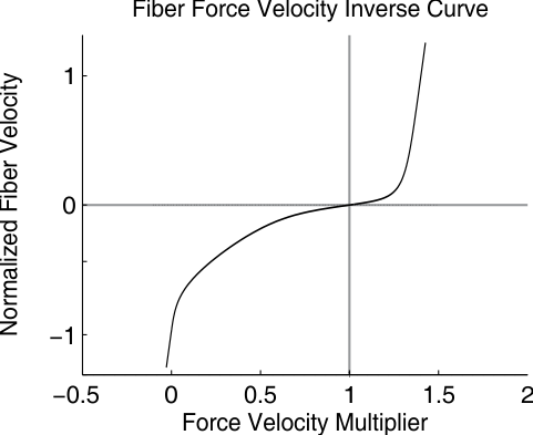
This function will generate a C2-continuous (continuous to the 2nd derivative) inverse curve that the function createFiberForceVelocityCurve generates.
The inverse force velocity curve is required by every equilibrium muscle model in order to compute the derivative of fiber velocity. To generate the inverse force velocity curve simply call this function with EXACTLY the same parameter values that you used to generate the force velocity curve. See the parameter descriptions for createFiberForceVelocityCurve, as the parameters for the inverse function are identical. The curve name should be different, however, because this is an inverse curve (e.g. "bicep_fiberForceVelocityInverseCurve")
|
static |
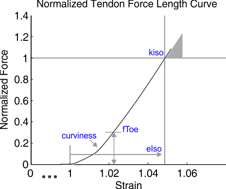
Will generate a C2-continuous (continuous to the second derivative) curve in a MuscleFunctionObject object that fits a tendon's tensile force length curve.
| eIso | The tendon strain at which the tendon develops 1 unit of normalized force (1 maximum isometric force). Note that the'1' is left off. Thus an e0 of 0.04 means that the tendon will develop an 1 normalized force unit when it is strained by 4% of its resting length, at a normalized length of 1.04 |
| kIso | The normalized stiffness (or slope) of the tendon curve when the tendon is strained by e0 (or has a length of 1+e0) under a load of 1 maximum isometric unit of force. |
| fToe | The normalized force at which the tendon smoothly transitions from the curved low stiffness region to the linear stiffness region. |
| curviness | The dimensionless 'curviness' parameter that can vary between 0 (a line) to 1 (a smooth, but sharply bent elbow) |
| computeIntegral | If this is true, the integral for this curve is numerically calculated and splined. If false, this integral is not computed, and a call to .calcIntegral will throw an exception |
| curveName | The name of the muscle this curve applies to. This curve name should have the name of the muscle and the curve in it (e.g. "bicep_tendonForceLengthCurve") so that, if this curve ever causes an exception, a user-friendly error message can be displayed to the end user to help them debug their model. |
| SimTK::Exception | unless the following conditions are met: -0 < fToe < 1 -e0 > 0 -kiso > 1/e0 -0 <= curviness <= 1 |
Computational Costs
    Without Integral :   ~4,100 flops
    With Integral    : ~174,100 flops
Example: